
This post presents a function mlReserve() for machine-learning loss reserving on ‘real-world’ triangles, based on a fork of R’s ‘ChainLadder’ package (https://github.com/thierrymoudiki/ChainLadder/tree/master). It includes two experiments, each scored against a known true reserve: (A) Two triangles from an individual-claims simulator (Wang & Wüthrich, https://github.com/actuarial-data-science/PackageIndividualClaimsSimulator), embedded below: chain ladder vs mlReserve, in detail; (B) A mini-benchmark on freshly simulated triangles from a simpler aggregate generator, with tunable distortions.
# =============================================================================
# mlReserve: machine-learning loss reserving on "real-world" triangles
#
# Colab: Runtime > Change runtime type > R
#
# Two experiments, each scored against a known true reserve:
#   A. Two triangles from an individual-claims simulator (Wang & Wüthrich),
#      embedded below: chain ladder vs mlReserve, in detail.
#   B. A mini-benchmark on freshly simulated triangles from a simpler aggregate
#      generator (defined in step 4), with tunable distortions.
# =============================================================================

# ---- 0. Setup -------------------------------------------------------------------

options(Ncpus = 2, repos = "https://cloud.r-project.org",
        repr.plot.width = 12, repr.plot.height = 5.5)
for (pkg in c("remotes", "ggplot2", "ranger", "e1071"))
  if (!requireNamespace(pkg, quietly = TRUE)) install.packages(pkg)
if (!requireNamespace("ChainLadder", quietly = TRUE) ||
    !"mlReserve" %in% getNamespaceExports("ChainLadder"))
  remotes::install_github("thierrymoudiki/ChainLadder", upgrade = "never")

suppressPackageStartupMessages({
  library(ChainLadder)
  library(ggplot2)
})

n      <- 10                                   # triangle size (accident years)
models <- c("Chain ladder", "mlReserve: SVM", "mlReserve: random forest")
ink    <- "#0b0b0b"
colours <- c("Chain ladder"             = "#eb6834",
             "mlReserve: SVM"           = "#2a78d6",
             "mlReserve: random forest" = "#1baf7a",
             "Truth"                    = ink)
theme_set(theme_minimal(base_size = 13) +
            theme(legend.position = "top", legend.title = element_blank(),
                  panel.grid.minor = element_blank(), plot.title.position = "plot",
                  strip.text = element_text(face = "bold")))


# ---- 1. Helpers -----------------------------------------------------------------

# A full n x n square of incremental payments -> observed (cumulative) upper
# triangle + true outstanding reserve per accident year (sum of the lower triangle)
make_case <- function(full) {
  dimnames(full) <- list(origin = 1:n, dev = 1:n)
  future <- row(full) + col(full) > n + 1
  upper  <- full; upper[future] <- NA
  list(full      = full,
       upper     = incr2cum(as.triangle(upper)),
       true_ibnr = rowSums(full * future))
}

# Fit the three models; `uncertainty = FALSE` gives point estimates only
fit_models <- function(triangle, uncertainty = TRUE, nsim = 300) {
  mse <- if (uncertainty) "bootstrap" else "none"
  fits <- list(
    MackChainLadder(triangle, est.sigma = "Mack"),
    mlReserve(triangle, e1071::svm, features = "numeric", transform = "asinh",
              mse.method = mse, nsim = nsim, seed = 1),
    mlReserve(triangle, ranger::ranger, num.trees = 300, num.threads = 1,
              features = "both", transform = "asinh",
              mse.method = mse, nsim = nsim, seed = 1))
  setNames(fits, models)
}

# Reserve (IBNR) and standard error by accident year, whatever the model
reserve_by_origin <- function(fit) {
  if (inherits(fit, "MackChainLadder")) {
    s <- summary(fit)$ByOrigin
    data.frame(origin = 1:n, IBNR = s$IBNR, SE = s$Mack.S.E)
  } else {
    s <- fit$summary[rownames(fit$summary) != "total", ]
    data.frame(origin = as.integer(rownames(s)), IBNR = s$IBNR, SE = s$S.E)
  }
}
total_reserve <- function(fit) sum(reserve_by_origin(fit)$IBNR)


# ---- 2. Data for experiment A ---------------------------------------------------

# Incremental paid (thousands), aggregated from the Wang & Wuthrich individual
# claims simulator (github.com/actuarial-data-science/PackageIndividualClaimsSimulator):
#   "Speed-up"     : settlement accelerates for recent accident years (delays -45%)
#   "All combined" : speed-up + calendar inflation shock (2% -> 15% a year from
#                    calendar month 78) + a few large, slowly paid claims
squares <- list(
  "Speed-up" = c(4172.1, 16153.4, 14800.2, 7561.1, 3275, 1856.3, 726.7, 410.7, 35.8, 140, 4983.2, 18064.1, 13574.5, 8350.7, 3954.9, 1499, 510.3, 9.5, 0, 11.3, 4698.1, 19428.8, 14864, 7343, 3710.5, 1378.6, 384.7, 92.2, 6.8, 27.1, 5467.1, 18481, 14847.6, 8089.7, 2794.1, 1379.2, 549.5, 152.2, 6.8, 0, 5985.2, 21516.6, 15980.6, 8353, 2954.2, 1655.5, 636.4, 191.3, 211.3, 28.9, 8274.1, 22014.4, 15981.4, 7425.8, 2362.7, 731, 242.1, 41.6, 52.8, 0, 8148.4, 24712.9, 16329.1, 6587.5, 2804.9, 753.6, 49.5, 0, 0, 0, 9974.2, 27573.4, 14523, 5141.6, 1123.8, 350, 73.3, 0, 0, 0, 10698.8, 29877.8, 14303.3, 3200.3, 978.3, 239.1, 0, 0, 0, 0, 13669.1, 30541.7, 10984, 1837.5, 157.3, 0, 0, 0, 0, 0),
  "All combined" = c(4236.8, 16766.9, 15671.5, 8229, 3582.8, 2143.9, 838.8, 548.6, 57.6, 261.6, 5195.7, 19008.8, 15926.9, 9857.6, 4643.8, 1746.5, 712.4, 26.4, 0, 22.5, 4956.8, 20861.6, 16283.4, 8704.2, 4321.7, 1876.2, 666.5, 161.8, 14.7, 61.4, 5908.2, 20336.4, 16580.1, 9331.1, 3673.8, 2276.2, 1205.8, 332.2, 15.4, 0, 6586.1, 24045.6, 18499, 11218.3, 4576, 3174.8, 1307, 460.6, 665, 96.3, 9292, 26084.3, 21055.7, 11396.7, 4203.8, 1531.8, 585.4, 115, 163.7, 0, 9702.9, 33010, 25202.7, 12133, 6404.4, 1956.8, 385.9, 0, 0, 0, 13752.5, 42686.8, 25857.7, 10698.4, 2706.5, 3213, 4232.5, 0, 0, 0, 17094.3, 53962.4, 30132.7, 8527.6, 3087.9, 746.2, 0, 0, 0, 0, 25375.8, 63473.7, 26195.3, 5737.2, 507, 674.2, 0, 0, 0, 0))
cases <- lapply(squares, function(v) make_case(matrix(v, n, n, byrow = TRUE)))
combo <- cases[["All combined"]]

cat("Observed cumulative paid, 'All combined' (thousands):\n")
print(round(combo$upper))
fits <- suppressWarnings(fit_models(combo$upper))
cat("\nmlReserve with a random forest; true total reserve =",
    format(round(sum(combo$true_ibnr)), big.mark = ","), "\n")
print(fits[["mlReserve: random forest"]])


# ---- 3. Experiment A: one triangle in detail ------------------------------------

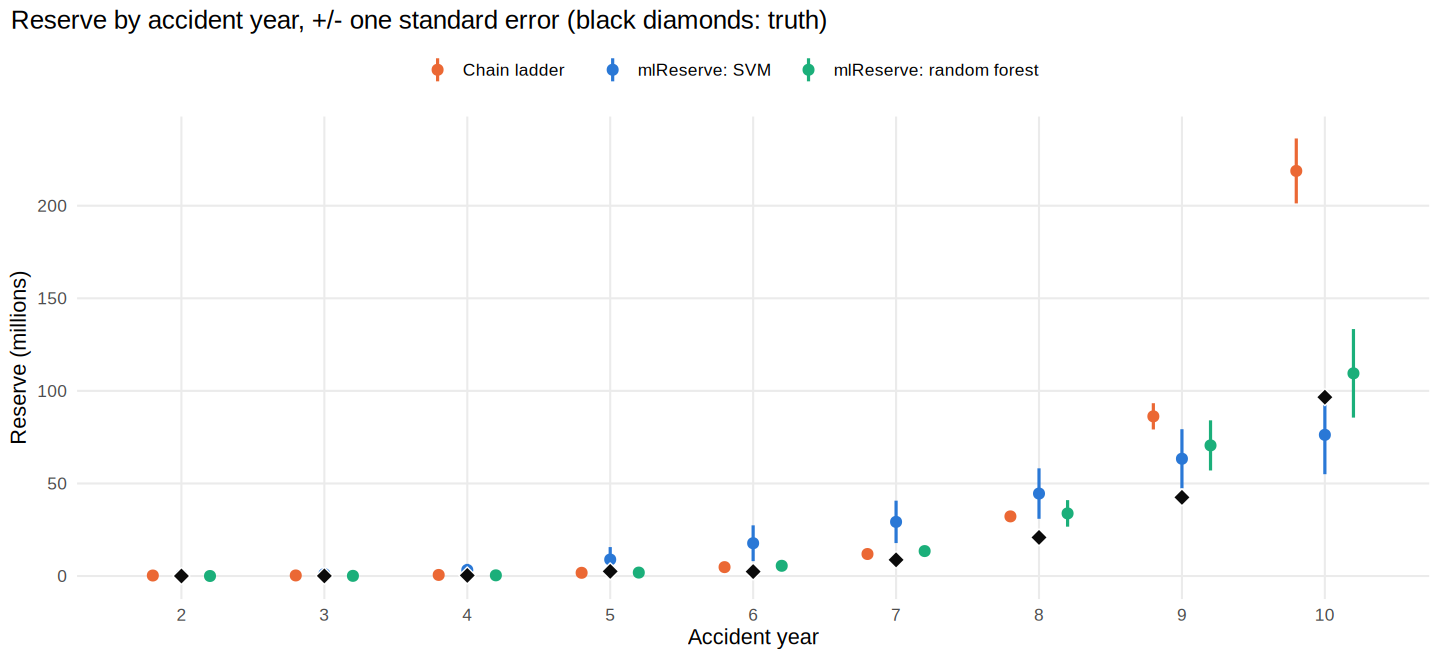
# 3a. Reserve by accident year vs the truth
by_origin <- do.call(rbind, lapply(models, function(m)
  data.frame(model = m, reserve_by_origin(fits[[m]]))))
by_origin <- subset(by_origin, origin >= 2)             # AY 1 is fully developed
by_origin$model <- factor(by_origin$model, levels = models)
truth_points <- data.frame(origin = 2:n, IBNR = combo$true_ibnr[2:n])

print(
  ggplot(by_origin, aes(origin, IBNR / 1000, colour = model)) +
    geom_linerange(aes(ymin = (IBNR - SE) / 1000, ymax = (IBNR + SE) / 1000),
                   position = position_dodge(0.6), linewidth = 0.9) +
    geom_point(position = position_dodge(0.6), size = 2.6) +
    geom_point(data = truth_points, aes(origin, IBNR / 1000), inherit.aes = FALSE,
               shape = 23, size = 3.4, fill = ink, colour = "white") +
    scale_colour_manual(values = colours) +
    scale_x_continuous(breaks = 2:n) +
    labs(title = "Reserve by accident year, +/- one standard error (black diamonds: truth)",
         x = "Accident year", y = "Reserve (millions)"))

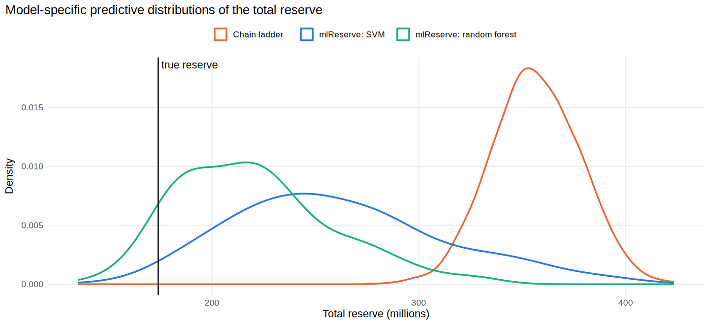
# 3b. Predictive distribution of the total reserve. Each model uses its own
#     resampling scheme: ODP bootstrap (BootChainLadder) for chain ladder,
#     residual bootstrap (mlReserve) for the learners.
set.seed(1)
boot <- BootChainLadder(combo$upper, R = 2000, process.distr = "od.pois")
draws <- rbind(
  data.frame(model = models[1], total = boot$IBNR.Totals),
  data.frame(model = models[2], total = rowSums(fits[[2]]$sims.reserve.pred)),
  data.frame(model = models[3], total = rowSums(fits[[3]]$sims.reserve.pred)))
draws$model <- factor(draws$model, levels = models)

print(
  ggplot(draws, aes(total / 1000, colour = model)) +
    geom_density(linewidth = 1, adjust = 1.2) +
    geom_vline(xintercept = sum(combo$true_ibnr) / 1000, colour = ink, linewidth = 0.8) +
    annotate("text", x = sum(combo$true_ibnr) / 1000, y = Inf, label = " true reserve",
             hjust = 0, vjust = 1.5, colour = ink) +
    scale_colour_manual(values = colours) +
    labs(title = "Model-specific predictive distributions of the total reserve",
         x = "Total reserve (millions)", y = "Density"))

cat("\nPredictive quantiles of the total reserve (thousands):\n")
quants <- t(sapply(split(draws$total, draws$model), quantile, c(0.025, 0.5, 0.975)))
print(noquote(formatC(round(quants), format = "d", big.mark = ",")))

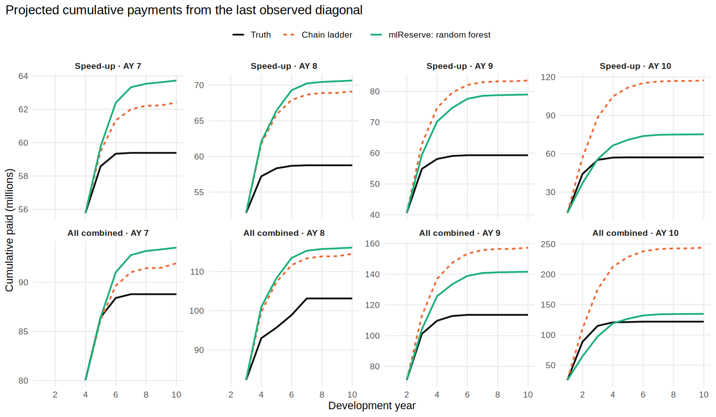
# 3c. Projected cumulative payments vs the truth, accident years 7-10
cumulative_paths <- function(case, label) {
  cl <- MackChainLadder(case$upper, est.sigma = "Mack")
  rf <- mlReserve(case$upper, ranger::ranger, num.trees = 300, num.threads = 1,
                  features = "both", transform = "asinh", mse.method = "none", seed = 1)
  projections <- list("Truth"                    = t(apply(case$full, 1, cumsum)),
                      "Chain ladder"             = unclass(cl$FullTriangle),
                      "mlReserve: random forest" = unclass(rf$FullTriangle))
  out <- expand.grid(dev = 1:n, origin = 7:n, model = names(projections),
                     stringsAsFactors = FALSE)
  out$value <- mapply(function(o, d, m) projections[[m]][o, d],
                      out$origin, out$dev, out$model)
  out$panel <- paste0(label, " · AY ", out$origin)
  subset(out, dev >= n + 1 - origin)      # from the last observed diagonal onwards
}
paths <- do.call(rbind, Map(cumulative_paths, cases, names(cases)))
paths$model <- factor(paths$model, levels = c("Truth", models[c(1, 3)]))
paths$panel <- factor(paths$panel, levels = unique(paths$panel))

options(repr.plot.height = 7)
print(
  ggplot(paths, aes(dev, value / 1000, colour = model, linetype = model)) +
    geom_line(linewidth = 1) +
    facet_wrap(~ panel, nrow = 2, scales = "free_y") +
    scale_colour_manual(values = colours) +
    scale_linetype_manual(values = c("solid", "22", "solid")) +
    scale_x_continuous(breaks = seq(2, n, 2)) +
    labs(title = "Projected cumulative payments from the last observed diagonal",
         x = "Development year", y = "Cumulative paid (millions)"))
options(repr.plot.height = 5.5)


# ---- 4. Experiment B: mini-benchmark on fresh triangles -------------------------

# Aggregate generator: gamma payment pattern with over-dispersed Poisson noise.
#   speedup   : mean payment delay shrinks by up to this share for recent AYs
#   inflation : calendar-year log-growth rate after calendar period 7 (2% before)
simulate_case <- function(seed, speedup = 0.3, inflation = 0.08, phi = 5) {
  set.seed(seed)
  ultimate <- 5e4 * (1 + 0.03 * (0:(n - 1))) * exp(rnorm(n, 0, 0.05))
  delay    <- 3 * (1 - speedup * pmax(0, (1:n - 4) / (n - 4)))
  pattern  <- t(sapply(delay, function(m) diff(pgamma(0:n, shape = 2, scale = m / 2))))
  calendar <- outer(1:n, 1:n, "+") - 1
  infl     <- exp(0.02 * pmin(calendar, 7) + inflation * pmax(calendar - 7, 0))
  mean_incr <- ultimate * pattern * infl
  make_case(phi * matrix(rpois(n * n, mean_incr / phi), n))
}

n_rep <- 20                                   # triangles per scenario
scenarios <- list(
  # "Baseline (no distortion)" = c(speedup = 0,   inflation = 0.02),  # control
  "Settlement speed-up"      = c(speedup = 0.3, inflation = 0.02),
  "Speed-up + inflation"     = c(speedup = 0.3, inflation = 0.08))

bench <- do.call(rbind, lapply(names(scenarios), function(sc) {
  do.call(rbind, lapply(seq_len(n_rep), function(seed) {
    case <- simulate_case(seed, speedup   = scenarios[[sc]][["speedup"]],
                                inflation = scenarios[[sc]][["inflation"]])
    point_fits <- suppressWarnings(fit_models(case$upper, uncertainty = FALSE))
    data.frame(scenario = sc, seed = seed, model = models,
               error = sapply(point_fits, total_reserve) - sum(case$true_ibnr))
  }))
}))

score <- aggregate(error ~ scenario + model, data = bench, FUN = function(e)
  c(bias = mean(e), RMSE = sqrt(mean(e^2)), MAE = mean(abs(e))))
score <- do.call(data.frame, score)
names(score) <- c("scenario", "model", "bias", "RMSE", "MAE")
score <- score[order(score$scenario, score$RMSE), ]

cat("\nError of the total reserve over", n_rep, "triangles per scenario (thousands):\n")
fmt <- function(x) formatC(round(x), format = "d", big.mark = ",")
print(transform(score, bias = fmt(bias), RMSE = fmt(RMSE), MAE = fmt(MAE)),
      row.names = FALSE)

long <- rbind(data.frame(score[c("scenario", "model")], metric = "RMSE", value = score$RMSE),
              data.frame(score[c("scenario", "model")], metric = "MAE",  value = score$MAE))
long$model <- factor(long$model, levels = rev(models))
print(
  ggplot(long, aes(value / 1000, model, fill = model)) +
    geom_col(width = 0.6) +
    facet_grid(metric ~ scenario, scales = "free_x") +
    scale_fill_manual(values = colours, guide = "none") +
    labs(title = "Out-of-sample error of the total reserve (lower is better)",
         x = "Millions", y = NULL))
Observed cumulative paid, 'All combined' (thousands):
      dev
origin     1     2     3     4     5     6     7     8     9    10
    1   4237 21004 36675 44904 48487 50631 51470 52018 52076 52338
    2   5196 24204 40131 49989 54633 56379 57092 57118 57118    NA
    3   4957 25818 42102 50806 55128 57004 57670 57832    NA    NA
    4   5908 26245 42825 52156 55830 58106 59312    NA    NA    NA
    5   6586 30632 49131 60349 64925 68100    NA    NA    NA    NA
    6   9292 35376 56432 67829 72032    NA    NA    NA    NA    NA
    7   9703 42713 67916 80049    NA    NA    NA    NA    NA    NA
    8  13752 56439 82297    NA    NA    NA    NA    NA    NA    NA
    9  17094 71057    NA    NA    NA    NA    NA    NA    NA    NA
    10 25376    NA    NA    NA    NA    NA    NA    NA    NA    NA

mlReserve with a random forest; true total reserve = 174,050
mlReserve (formula interface)

        Latest Dev.To.Date Ultimate   IBNR         S.E        CV
2      57118.1   0.9994925  57147.1     29    39.76128 1.3710786
3      57832.2   0.9982222  57935.2    103    91.80065 0.8912685
4      59311.6   0.9935674  59695.6    384   244.97640 0.6379594
5      68099.8   0.9732881  69968.8   1869   888.80702 0.4755522
6      72032.5   0.9286787  77564.5   5532  1605.55443 0.2902304
7      80048.6   0.8558364  93532.6  13484  2443.15573 0.1811892
8      82297.0   0.7087359 116118.0  33821  7158.48746 0.2116581
9      71056.7   0.5017785 141609.7  70553 13547.27988 0.1920156
10     25375.8   0.1881838 134845.8 109470 23912.17707 0.2184359
total 573172.3   0.7090055 808417.3 235245 37338.60673 0.1587222
Predictive quantiles of the total reserve (thousands):
                         2.5%    50%     97.5%
Chain ladder             316,100 356,087 397,519
mlReserve: SVM           178,587 252,035 371,639
mlReserve: random forest 162,579 217,369 301,946
Error of the total reserve over 20 triangles per scenario (thousands):
             scenario                    model    bias    RMSE     MAE
  Settlement speed-up mlReserve: random forest  67,436  67,519  67,436
  Settlement speed-up             Chain ladder  94,022  94,097  94,022
  Settlement speed-up           mlReserve: SVM  93,888  94,318  93,888
 Speed-up + inflation mlReserve: random forest  58,834  58,975  58,834
 Speed-up + inflation           mlReserve: SVM  79,344  79,800  79,344
 Speed-up + inflation             Chain ladder 100,217 100,311 100,217
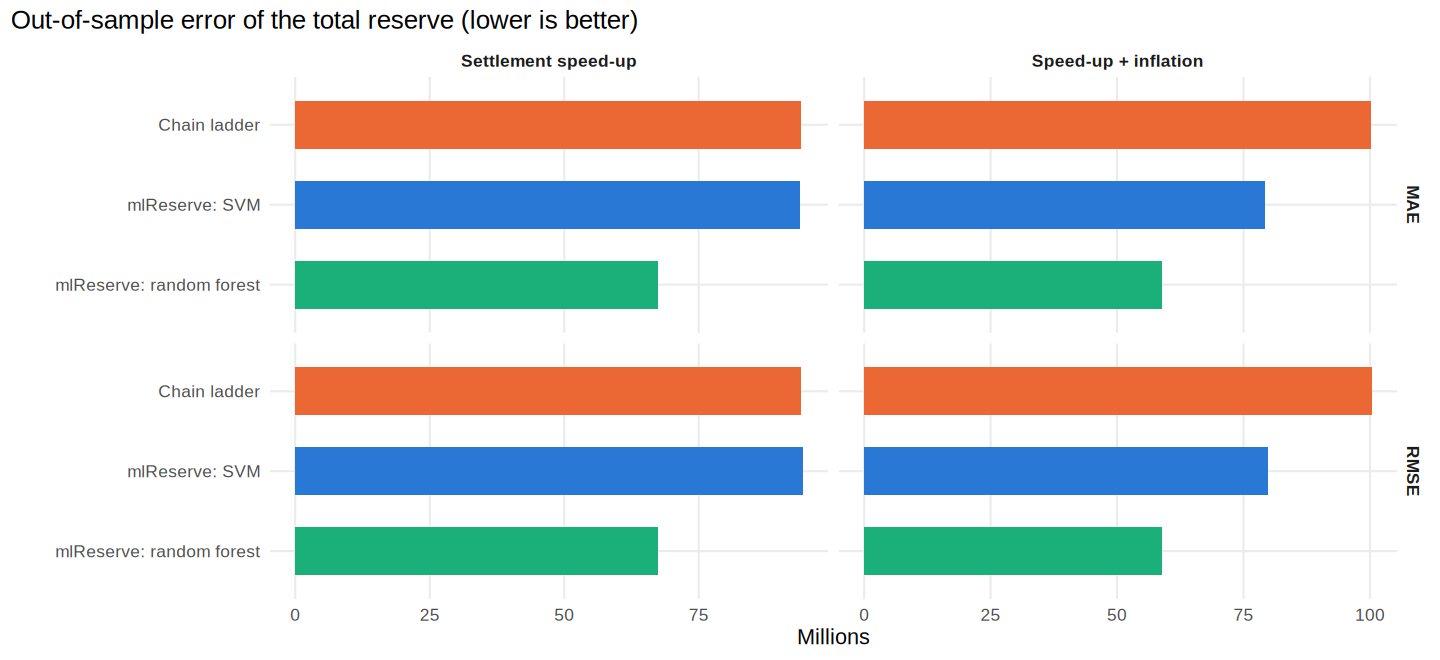
The experiment is not a universal proof that random forests are better. It is a demonstration that mlReserve() can be used to explore the performance of machine-learning models on loss reserving problems, and that it can outperform the classical chain ladder method in some scenarios.
For attribution, please cite this work as:
T. Moudiki (2026-10-03). mlreserve: machine-learning loss reserving on 'real-world' triangles (based on a 'ChainLadder' fork). Retrieved from https://thierrymoudiki.github.io/blog/2026/10/03/r/mlreserve
BibTeX citation (remove empty spaces)
        @misc{ tmoudiki20261003,
          author = { T. Moudiki },
          title = { mlreserve: machine-learning loss reserving on 'real-world' triangles (based on a 'ChainLadder' fork) },
          url = { https://thierrymoudiki.github.io/blog/2026/10/03/r/mlreserve },
          year = { 2026 } }

Previous publications
- Choosing the size of the calibration set in conformal prediction with ahead::conformalize() Oct 18, 2026
- Machine-learning loss reserving vs Mack Chain-Ladder under settlement speed-up and calendar inflation (Python version) Oct 5, 2026
- mlreserve: machine-learning loss reserving on 'real-world' triangles (based on a 'ChainLadder' fork) Oct 3, 2026
- Analytics Pipeline for Dashboards, with Python, R and Javascript Sep 27, 2026
- Python version of Semi-parametric option pricing based on underlying's historical data (accepted at the osQF 2026 (ex R/Finance) conference) Sep 21, 2026
- Semi-parametric option pricing based on underlying's historical data (accepted at the osQF 2026 (ex R/Finance) conference) Sep 20, 2026
- Model-agnostic prediction intervals in Python and R: does nnetsauce's QuantileRegressor hold up? Sep 14, 2026
- ahead (Time Series Forecasting with uncertainty quantification) gets a lot faster to install: most dependencies are now optional Sep 8, 2026
- Skip the R/Python runtime: fast tabular dashboards with Observable Framework Aug 31, 2026
- PCARVFL vs CTGAN for synthetic tabular data generation on an insurance pricing dataset Aug 22, 2026
- 'Zero-Shot Probabilistic Stock Returns Forecasting with Pretrained RVFL Networks' accepted at COPA 2026 (and to appear in the Proceedings of Machine Learning Research) Aug 15, 2026
- 'PCARVFLSimulator': a GAN-like tabular data synthesizer built from PCA scores, a Random Vector Functional-Link network, and residuals bootstrapping Aug 10, 2026
- 'garchf': GARCH probabilistic forecasting with package 'forecast'-style interface (and 'rugarch' under the hood) Aug 1, 2026
- GPopt for R: Bayesian and conformal optimization of black-box functions and hyperparameter tuning Jul 26, 2026
- My last R posts: How conformalization helps weak models, fast conformal prediction with jackknife+ (and no refitting), and sklearn in R Jul 13, 2026
- Natively Interpretable Boosting Jul 12, 2026
- Fast conformal prediction (no refitting) for some Machine Learning models via closed-form jackknife plus Jun 27, 2026
- Using scikit-learn models in R easily with the tisthemachinelearner package Jun 21, 2026
- No-Code Machine Learning in Excel with the Techtonique API Jun 14, 2026
- How Conformal Prediction Makes Linear Models Good Enough — An Example Using R Package mlS3 Jun 7, 2026
- Techtonique dot net, the Machine Learning web API, is back online (but more like a passion project for now) May 31, 2026
- Conformalized TabICL: Prediction Intervals for a State-Of-The-Art Tabular Foundation Model in Python and R May 21, 2026
- Conformalized TabPFN: Prediction Intervals for a Pretrained Transformer for Tabular Data in Python and R May 17, 2026
- Probabilistic Time Series Cross-Validation with R package crossvalidation May 16, 2026
- One interface, (Almost) Every Classifier (and Regressor): unifiedml v0.3.0 May 9, 2026
- You Don't Need to Learn All the Weights on tabular data: The Case for rvflnet (a nonlinear expressive glmnet) on regression, classification and survival analysis May 2, 2026
- Survival analysis with sklearn, glmnet, keras, pytorch, lightgbm, xgboost, nnetsauce, mlsauce Part 2 Apr 28, 2026
- Any Sklearn Regressor as a Survival Model — Does It Actually Work? Benchmarking vs Established Packages Apr 26, 2026
- Conformal Optimization Beats Bayesian Optimization, Optuna and Random Search on 72 classification Datasets Apr 19, 2026
- `mlS3` — A Unified S3 Machine Learning Interface in R Apr 12, 2026
- One interface, (Almost) Every Classifier: unifiedml v0.2.1 Apr 4, 2026
- Techtonique dot net is down until further notice Apr 1, 2026
- Explaining Time-Series Forecasts with Sensitivity Analysis (ahead::dynrmf and external regressors) Mar 29, 2026
- Python version of 'Option pricing using time series models as market price of risk Pt.3' Mar 22, 2026
- Option pricing using time series models as market price of risk Pt.3 Mar 16, 2026
- Explaining Time-Series Forecasts with Exact Shapley Values (ahead::dynrmf with external regressors applied to scenarios) Mar 8, 2026
- My Presentation at Risk 2026: Lightweight Transfer Learning for Financial Forecasting Mar 1, 2026
- nnetsauce with and without jax for GPU acceleration Feb 23, 2026
- Understanding Boosted Configuration Networks (combined neural networks and boosting): An Intuitive Guide Through Their Hyperparameters Feb 16, 2026
- R version of Python package survivalist, for model-agnostic survival analysis Feb 9, 2026
- Presenting Lightweight Transfer Learning for Financial Forecasting (Risk 2026) Feb 4, 2026
- Option pricing using time series models as market price of risk Feb 1, 2026
- Enhancing Time Series Forecasting (ahead::ridge2f) with Attention-Based Context Vectors (ahead::contextridge2f) Jan 31, 2026
- Overfitting and scaling (on GPU T4) tests on nnetsauce.CustomRegressor Jan 29, 2026
- Beyond Cross-validation: Hyperparameter Optimization via Generalization Gap Modeling Jan 25, 2026
- GPopt for Machine Learning (hyperparameters' tuning) Jan 21, 2026
- rtopy: an R to Python bridge -- novelties Jan 8, 2026
- Python examples for 'Beyond Nelson-Siegel and splines: A model- agnostic Machine Learning framework for discount curve calibration, interpolation and extrapolation' Jan 3, 2026
- Forecasting benchmark: Dynrmf (a new serious competitor in town) vs Theta Method on M-Competitions and Tourism competitition Jan 1, 2026
- Finally figured out a way to port python packages to R using uv and reticulate: example with nnetsauce Dec 17, 2025
- Overfitting Random Fourier Features: Universal Approximation Property Dec 13, 2025
- Counterfactual Scenario Analysis with ahead::ridge2f Dec 11, 2025
- Zero-Shot Probabilistic Time Series Forecasting with TabPFN 2.5 and nnetsauce Dec 10, 2025
- ARIMA Pricing: Semi-Parametric Market price of risk for Risk-Neutral Pricing (code + preprint) Dec 7, 2025
- Analyzing Paper Reviews with LLMs: I Used ChatGPT, DeepSeek, Qwen, Mistral, Gemini, and Claude (and you should too + publish the analysis) Dec 3, 2025
- tisthemachinelearner: New Workflow with uv for R Integration of scikit-learn Dec 1, 2025
- (ICYMI) RPweave: Unified R + Python + LaTeX System using uv Nov 21, 2025
- unifiedml: A Unified Machine Learning Interface for R, is now on CRAN + Discussion about AI replacing humans Nov 16, 2025
- Context-aware Theta forecasting Method: Extending Classical Time Series Forecasting with Machine Learning Nov 13, 2025
- unifiedml in R: A Unified Machine Learning Interface Nov 5, 2025
- Deterministic Shift Adjustment in Arbitrage-Free Pricing (historical to risk-neutral short rates) Oct 28, 2025
- New instantaneous short rates models with their deterministic shift adjustment, for historical and risk-neutral simulation Oct 27, 2025
- RPweave: Unified R + Python + LaTeX System using uv Oct 19, 2025
- GAN-like Synthetic Data Generation Examples (on univariate, multivariate distributions, digits recognition, Fashion-MNIST, stock returns, and Olivetti faces) with DistroSimulator Oct 19, 2025
- R port of llama2.c Oct 9, 2025
- Native uncertainty quantification for time series with NGBoost Oct 8, 2025
- NGBoost (Natural Gradient Boosting) for Regression, Classification, Time Series forecasting and Reserving Oct 6, 2025
- Real-time pricing with a pretrained probabilistic stock return model Oct 1, 2025
- Combining any model with GARCH(1,1) for probabilistic stock forecasting Sep 23, 2025
- Generating Synthetic Data with R-vine Copulas using esgtoolkit in R Sep 21, 2025
- Reimagining Equity Solvency Capital Requirement Approximation (one of my Master's Thesis subjects): From Bilinear Interpolation to Probabilistic Machine Learning Sep 16, 2025
- Transfer Learning using ahead::ridge2f on synthetic stocks returns Pt.2: synthetic data generation Sep 9, 2025
- Transfer Learning using ahead::ridge2f on synthetic stocks returns Sep 8, 2025
- I'm supposed to present 'Conformal Predictive Simulations for Univariate Time Series' at COPA CONFERENCE 2025 in London... Sep 4, 2025
- external regressors in ahead::dynrmf's interface for Machine learning forecasting Sep 1, 2025
- Another interesting decision, now for 'Beyond Nelson-Siegel and splines: A model-agnostic Machine Learning framework for discount curve calibration, interpolation and extrapolation' Aug 20, 2025
- Boosting any randomized based learner for regression, classification and univariate/multivariate time series forcasting Jul 26, 2025
- New nnetsauce version with CustomBackPropRegressor (CustomRegressor with Backpropagation) and ElasticNet2Regressor (Ridge2 with ElasticNet regularization) Jul 15, 2025
- mlsauce (home to a model-agnostic gradient boosting algorithm) can now be installed from PyPI. Jul 10, 2025
- A user-friendly graphical interface to techtonique dot net's API (will eventually contain graphics). Jul 8, 2025
- Calling =TECHTO_MLCLASSIFICATION for Machine Learning supervised CLASSIFICATION in Excel is just a matter of copying and pasting Jul 7, 2025
- Calling =TECHTO_MLREGRESSION for Machine Learning supervised regression in Excel is just a matter of copying and pasting Jul 6, 2025
- Calling =TECHTO_RESERVING and =TECHTO_MLRESERVING for claims triangle reserving in Excel is just a matter of copying and pasting Jul 5, 2025
- Calling =TECHTO_SURVIVAL for Survival Analysis in Excel is just a matter of copying and pasting Jul 4, 2025
- Calling =TECHTO_SIMULATION for Stochastic Simulation in Excel is just a matter of copying and pasting Jul 3, 2025
- Calling =TECHTO_FORECAST for forecasting in Excel is just a matter of copying and pasting Jul 2, 2025
- Random Vector Functional Link (RVFL) artificial neural network with 2 regularization parameters successfully used for forecasting/synthetic simulation in professional settings: Extensions (including Bayesian) Jul 1, 2025
- R version of 'Backpropagating quasi-randomized neural networks' Jun 24, 2025
- Backpropagating quasi-randomized neural networks Jun 23, 2025
- Beyond ARMA-GARCH: leveraging any statistical model for volatility forecasting Jun 21, 2025
- Stacked generalization (Machine Learning model stacking) + conformal prediction for forecasting with ahead::mlf Jun 18, 2025
- An Overfitting dilemma: XGBoost Default Hyperparameters vs GenericBooster + LinearRegression Default Hyperparameters Jun 14, 2025
- Programming language-agnostic reserving using RidgeCV, LightGBM, XGBoost, and ExtraTrees Machine Learning models Jun 13, 2025
- Free R, Python and SQL editors in techtonique dot net Jun 9, 2025
- Beyond Nelson-Siegel and splines: A model-agnostic Machine Learning framework for discount curve calibration, interpolation and extrapolation Jun 7, 2025
- scikit-learn, glmnet, xgboost, lightgbm, pytorch, keras, nnetsauce in probabilistic Machine Learning (for longitudinal data) Reserving (work in progress) Jun 6, 2025
- R version of Probabilistic Machine Learning (for longitudinal data) Reserving (work in progress) Jun 5, 2025
- Probabilistic Machine Learning (for longitudinal data) Reserving (work in progress) Jun 4, 2025
- Python version of Beyond ARMA-GARCH: leveraging model-agnostic Quasi-Randomized networks and conformal prediction for nonparametric probabilistic stock forecasting (ML-ARCH) Jun 3, 2025
- Beyond ARMA-GARCH: leveraging model-agnostic Machine Learning and conformal prediction for nonparametric probabilistic stock forecasting (ML-ARCH) Jun 2, 2025
- Permutations and SHAPley values for feature importance in techtonique dot net's API (with R + Python + the command line) Jun 1, 2025
- Which patient is going to survive longer? Another guide to using techtonique dot net's API (with R + Python + the command line) for survival analysis May 31, 2025
- A Guide to Using techtonique.net's API and rush for simulating and plotting Stochastic Scenarios May 30, 2025
- Simulating Stochastic Scenarios with Diffusion Models: A Guide to Using techtonique.net's API for the purpose May 29, 2025
- Will my apartment in 5th avenue be overpriced or not? Harnessing the power of www.techtonique.net (+ xgboost, lightgbm, catboost) to find out May 28, 2025
- How long must I wait until something happens: A Comprehensive Guide to Survival Analysis via an API May 27, 2025
- Harnessing the Power of techtonique.net: A Comprehensive Guide to Machine Learning Classification via an API May 26, 2025
- Quantile regression with any regressor -- Examples with RandomForestRegressor, RidgeCV, KNeighborsRegressor May 20, 2025
- Survival stacking: survival analysis translated as supervised classification in R and Python May 5, 2025
- 'Bayesian' optimization of hyperparameters in a R machine learning model using the bayesianrvfl package Apr 25, 2025
- A lightweight interface to scikit-learn in R: Bayesian and Conformal prediction Apr 21, 2025
- A lightweight interface to scikit-learn in R Pt.2: probabilistic time series forecasting in conjunction with ahead::dynrmf Apr 20, 2025
- Extending the Theta forecasting method to GLMs, GAMs, GLMBOOST and attention: benchmarking on Tourism, M1, M3 and M4 competition data sets (28000 series) Apr 14, 2025
- Extending the Theta forecasting method to GLMs and attention Apr 8, 2025
- Nonlinear conformalized Generalized Linear Models (GLMs) with R package 'rvfl' (and other models) Mar 31, 2025
- Probabilistic Time Series Forecasting (predictive simulations) in Microsoft Excel using Python, xlwings lite and www.techtonique.net Mar 28, 2025
- Conformalize (improved prediction intervals and simulations) any R Machine Learning model with misc::conformalize Mar 25, 2025
- My poster for the 18th FINANCIAL RISKS INTERNATIONAL FORUM by Institut Louis Bachelier/Fondation du Risque/Europlace Institute of Finance Mar 19, 2025
- Interpretable probabilistic kernel ridge regression using Matérn 3/2 kernels Mar 16, 2025
- (News from) Probabilistic Forecasting of univariate and multivariate Time Series using Quasi-Randomized Neural Networks (Ridge2) and Conformal Prediction Mar 9, 2025
- Word-Online: re-creating Karpathy's char-RNN (with supervised linear online learning of word embeddings) for text completion Mar 8, 2025
- CRAN-like repository for most recent releases of Techtonique's R packages Mar 2, 2025
- Presenting 'Online Probabilistic Estimation of Carbon Beta and Carbon Shapley Values for Financial and Climate Risk' at Institut Louis Bachelier Feb 27, 2025
- Web app with DeepSeek R1 and Hugging Face API for chatting Feb 23, 2025
- tisthemachinelearner: A Lightweight interface to scikit-learn with 2 classes, Classifier and Regressor (in Python and R) Feb 17, 2025
- R version of survivalist: Probabilistic model-agnostic survival analysis using scikit-learn, xgboost, lightgbm (and conformal prediction) Feb 12, 2025
- Model-agnostic global Survival Prediction of Patients with Myeloid Leukemia in QRT/Gustave Roussy Challenge (challengedata.ens.fr): Python's survivalist Quickstart Feb 10, 2025
- A simple test of the martingale hypothesis in esgtoolkit Feb 3, 2025
- Command Line Interface (CLI) for techtonique.net's API Jan 31, 2025
- Gradient-Boosting and Boostrap aggregating anything (alert: high performance): Part5, easier install and Rust backend Jan 27, 2025
- Just got a paper on conformal prediction REJECTED by International Journal of Forecasting despite evidence on 30,000 time series (and more). What's going on? Part2: 1311 time series from the Tourism competition Jan 20, 2025
- Techtonique is released! (with a tutorial in various programming languages and formats) Jan 14, 2025
- Univariate and Multivariate Probabilistic Forecasting with nnetsauce and TabPFN Jan 14, 2025
- Just got a paper on conformal prediction REJECTED by International Journal of Forecasting despite evidence on 30,000 time series (and more). What's going on? Jan 5, 2025
- Python and Interactive dashboard version of Stock price forecasting with Deep Learning: throwing power at the problem (and why it won't make you rich) Dec 31, 2024
- Stock price forecasting with Deep Learning: throwing power at the problem (and why it won't make you rich) Dec 29, 2024
- No-code Machine Learning Cross-validation and Interpretability in techtonique.net Dec 23, 2024
- survivalist: Probabilistic model-agnostic survival analysis using scikit-learn, glmnet, xgboost, lightgbm, pytorch, keras, nnetsauce and mlsauce Dec 15, 2024
- Model-agnostic 'Bayesian' optimization (for hyperparameter tuning) using conformalized surrogates in GPopt Dec 9, 2024
- You can beat Forecasting LLMs (Large Language Models a.k.a foundation models) with nnetsauce.MTS Pt.2: Generic Gradient Boosting Dec 1, 2024
- You can beat Forecasting LLMs (Large Language Models a.k.a foundation models) with nnetsauce.MTS Nov 24, 2024
- Unified interface and conformal prediction (calibrated prediction intervals) for R package forecast (and 'affiliates') Nov 23, 2024
- GLMNet in Python: Generalized Linear Models Nov 18, 2024
- Gradient-Boosting anything (alert: high performance): Part4, Time series forecasting Nov 10, 2024
- Predictive scenarios simulation in R, Python and Excel using Techtonique API Nov 3, 2024
- Chat with your tabular data in www.techtonique.net Oct 30, 2024
- Gradient-Boosting anything (alert: high performance): Part3, Histogram-based boosting Oct 28, 2024
- R editor and SQL console (in addition to Python editors) in www.techtonique.net Oct 21, 2024
- R and Python consoles + JupyterLite in www.techtonique.net Oct 15, 2024
- Gradient-Boosting anything (alert: high performance): Part2, R version Oct 14, 2024
- Gradient-Boosting anything (alert: high performance) Oct 6, 2024
- Benchmarking 30 statistical/Machine Learning models on the VN1 Forecasting -- Accuracy challenge Oct 4, 2024
- Automated random variable distribution inference using Kullback-Leibler divergence and simulating best-fitting distribution Oct 2, 2024
- Forecasting in Excel using Techtonique's Machine Learning APIs under the hood Sep 30, 2024
- Techtonique web app for data-driven decisions using Mathematics, Statistics, Machine Learning, and Data Visualization Sep 25, 2024
- Parallel for loops (Map or Reduce) + New versions of nnetsauce and ahead Sep 16, 2024
- Adaptive (online/streaming) learning with uncertainty quantification using Polyak averaging in learningmachine Sep 10, 2024
- New versions of nnetsauce and ahead Sep 9, 2024
- Prediction sets and prediction intervals for conformalized Auto XGBoost, Auto LightGBM, Auto CatBoost, Auto GradientBoosting Sep 2, 2024
- Quick/automated R package development workflow (assuming you're using macOS or Linux) Part2 Aug 30, 2024
- R package development workflow (assuming you're using macOS or Linux) Aug 27, 2024
- A new method for deriving a nonparametric confidence interval for the mean Aug 26, 2024
- Conformalized adaptive (online/streaming) learning using learningmachine in Python and R Aug 19, 2024
- Bayesian (nonlinear) adaptive learning Aug 12, 2024
- Auto XGBoost, Auto LightGBM, Auto CatBoost, Auto GradientBoosting Aug 5, 2024
- Copulas for uncertainty quantification in time series forecasting Jul 28, 2024
- Forecasting uncertainty: sequential split conformal prediction + Block bootstrap (web app) Jul 22, 2024
- learningmachine for Python (new version) Jul 15, 2024
- learningmachine v2.0.0: Machine Learning with explanations and uncertainty quantification Jul 8, 2024
- My presentation at ISF 2024 conference (slides with nnetsauce probabilistic forecasting news) Jul 3, 2024
- 10 uncertainty quantification methods in nnetsauce forecasting Jul 1, 2024
- Forecasting with XGBoost embedded in Quasi-Randomized Neural Networks Jun 24, 2024
- Forecasting Monthly Airline Passenger Numbers with Quasi-Randomized Neural Networks Jun 17, 2024
- Automated hyperparameter tuning using any conformalized surrogate Jun 9, 2024
- Recognizing handwritten digits with Ridge2Classifier Jun 3, 2024
- Forecasting the Economy May 27, 2024
- A detailed introduction to Deep Quasi-Randomized 'neural' networks May 19, 2024
- Probability of receiving a loan; using learningmachine May 12, 2024
- mlsauce's `v0.18.2`: various examples and benchmarks with dimension reduction May 6, 2024
- mlsauce's `v0.17.0`: boosting with Elastic Net, polynomials and heterogeneity in explanatory variables Apr 29, 2024
- mlsauce's `v0.13.0`: taking into account inputs heterogeneity through clustering Apr 21, 2024
- mlsauce's `v0.12.0`: prediction intervals for LSBoostRegressor Apr 15, 2024
- Conformalized predictive simulations for univariate time series on more than 250 data sets Apr 7, 2024
- learningmachine v1.1.2: for Python Apr 1, 2024
- learningmachine v1.0.0: prediction intervals around the probability of the event 'a tumor being malignant' Mar 25, 2024
- Bayesian inference and conformal prediction (prediction intervals) in nnetsauce v0.18.1 Mar 18, 2024
- Multiple examples of Machine Learning forecasting with ahead Mar 11, 2024
- rtopy (v0.1.1): calling R functions in Python Mar 4, 2024
- ahead forecasting (v0.10.0): fast time series model calibration and Python plots Feb 26, 2024
- A plethora of datasets at your fingertips Part3: how many times do couples cheat on each other? Feb 19, 2024
- nnetsauce's introduction as of 2024-02-11 (new version 0.17.0) Feb 11, 2024
- Tuning Machine Learning models with GPopt's new version Part 2 Feb 5, 2024
- Tuning Machine Learning models with GPopt's new version Jan 29, 2024
- Subsampling continuous and discrete response variables Jan 22, 2024
- DeepMTS, a Deep Learning Model for Multivariate Time Series Jan 15, 2024
- A classifier that's very accurate (and deep) Pt.2: there are > 90 classifiers in nnetsauce Jan 8, 2024
- learningmachine: prediction intervals for conformalized Kernel ridge regression and Random Forest Jan 1, 2024
- A plethora of datasets at your fingertips Part2: how many times do couples cheat on each other? Descriptive analytics, interpretability and prediction intervals using conformal prediction Dec 25, 2023
- Diffusion models in Python with esgtoolkit (Part2) Dec 18, 2023
- Diffusion models in Python with esgtoolkit Dec 11, 2023
- Julia packaging at the command line Dec 4, 2023
- Quasi-randomized nnetworks in Julia, Python and R Nov 27, 2023
- A plethora of datasets at your fingertips Nov 20, 2023
- A classifier that's very accurate (and deep) Nov 12, 2023
- mlsauce version 0.8.10: Statistical/Machine Learning with Python and R Nov 5, 2023
- AutoML in nnetsauce (randomized and quasi-randomized nnetworks) Pt.2: multivariate time series forecasting Oct 29, 2023
- AutoML in nnetsauce (randomized and quasi-randomized nnetworks) Oct 22, 2023
- Version v0.14.0 of nnetsauce for R and Python Oct 16, 2023
- A diffusion model: G2++ Oct 9, 2023
- Diffusion models in ESGtoolkit + announcements Oct 2, 2023
- An infinity of time series forecasting models in nnetsauce (Part 2 with uncertainty quantification) Sep 25, 2023
- (News from) forecasting in Python with ahead (progress bars and plots) Sep 18, 2023
- Forecasting in Python with ahead Sep 11, 2023
- Risk-neutralize simulations Sep 4, 2023
- Comparing cross-validation results using crossval_ml and boxplots Aug 27, 2023
- Reminder Apr 30, 2023
- Did you ask ChatGPT about who you are? Apr 16, 2023
- A new version of nnetsauce (randomized and quasi-randomized 'neural' networks) Apr 2, 2023
- Simple interfaces to the forecasting API Nov 23, 2022
- A web application for forecasting in Python, R, Ruby, C#, JavaScript, PHP, Go, Rust, Java, MATLAB, etc. Nov 2, 2022
- Prediction intervals (not only) for Boosted Configuration Networks in Python Oct 5, 2022
- Boosted Configuration (neural) Networks Pt. 2 Sep 3, 2022
- Boosted Configuration (_neural_) Networks for classification Jul 21, 2022
- A Machine Learning workflow using Techtonique Jun 6, 2022
- Super Mario Bros © in the browser using PyScript May 8, 2022
- News from ESGtoolkit, ycinterextra, and nnetsauce Apr 4, 2022
- Explaining a Keras _neural_ network predictions with the-teller Mar 11, 2022
- New version of nnetsauce -- various quasi-randomized networks Feb 12, 2022
- A dashboard illustrating bivariate time series forecasting with `ahead` Jan 14, 2022
- Hundreds of Statistical/Machine Learning models for univariate time series, using ahead, ranger, xgboost, and caret Dec 20, 2021
- Forecasting with `ahead` (Python version) Dec 13, 2021
- Tuning and interpreting LSBoost Nov 15, 2021
- Time series cross-validation using `crossvalidation` (Part 2) Nov 7, 2021
- Fast and scalable forecasting with ahead::ridge2f Oct 31, 2021
- Automatic Forecasting with `ahead::dynrmf` and Ridge regression Oct 22, 2021
- Forecasting with `ahead` Oct 15, 2021
- Classification using linear regression Sep 26, 2021
- `crossvalidation` and random search for calibrating support vector machines Aug 6, 2021
- parallel grid search cross-validation using `crossvalidation` Jul 31, 2021
- `crossvalidation` on R-universe, plus a classification example Jul 23, 2021
- Documentation and source code for GPopt, a package for Bayesian optimization Jul 2, 2021
- Hyperparameters tuning with GPopt Jun 11, 2021
- A forecasting tool (API) with examples in curl, R, Python May 28, 2021
- Bayesian Optimization with GPopt Part 2 (save and resume) Apr 30, 2021
- Bayesian Optimization with GPopt Apr 16, 2021
- Compatibility of nnetsauce and mlsauce with scikit-learn Mar 26, 2021
- Explaining xgboost predictions with the teller Mar 12, 2021
- An infinity of time series models in nnetsauce Mar 6, 2021
- New activation functions in mlsauce's LSBoost Feb 12, 2021
- 2020 recap, Gradient Boosting, Generalized Linear Models, AdaOpt with nnetsauce and mlsauce Dec 29, 2020
- A deeper learning architecture in nnetsauce Dec 18, 2020
- Classify penguins with nnetsauce's MultitaskClassifier Dec 11, 2020
- Bayesian forecasting for uni/multivariate time series Dec 4, 2020
- Generalized nonlinear models in nnetsauce Nov 28, 2020
- Boosting nonlinear penalized least squares Nov 21, 2020
- Statistical/Machine Learning explainability using Kernel Ridge Regression surrogates Nov 6, 2020
- NEWS Oct 30, 2020
- A glimpse into my PhD journey Oct 23, 2020
- Submitting R package to CRAN Oct 16, 2020
- Simulation of dependent variables in ESGtoolkit Oct 9, 2020
- Forecasting lung disease progression Oct 2, 2020
- New nnetsauce Sep 25, 2020
- Technical documentation Sep 18, 2020
- A new version of nnetsauce, and a new Techtonique website Sep 11, 2020
- Back next week, and a few announcements Sep 4, 2020
- Explainable 'AI' using Gradient Boosted randomized networks Pt2 (the Lasso) Jul 31, 2020
- LSBoost: Explainable 'AI' using Gradient Boosted randomized networks (with examples in R and Python) Jul 24, 2020
- nnetsauce version 0.5.0, randomized neural networks on GPU Jul 17, 2020
- Maximizing your tip as a waiter (Part 2) Jul 10, 2020
- New version of mlsauce, with Gradient Boosted randomized networks and stump decision trees Jul 3, 2020
- Announcements Jun 26, 2020
- Parallel AdaOpt classification Jun 19, 2020
- Comments section and other news Jun 12, 2020
- Maximizing your tip as a waiter Jun 5, 2020
- AdaOpt classification on MNIST handwritten digits (without preprocessing) May 29, 2020
- AdaOpt (a probabilistic classifier based on a mix of multivariable optimization and nearest neighbors) for R May 22, 2020
- AdaOpt May 15, 2020
- Custom errors for cross-validation using crossval::crossval_ml May 8, 2020
- Documentation+Pypi for the `teller`, a model-agnostic tool for Machine Learning explainability May 1, 2020
- Encoding your categorical variables based on the response variable and correlations Apr 24, 2020
- Linear model, xgboost and randomForest cross-validation using crossval::crossval_ml Apr 17, 2020
- Grid search cross-validation using crossval Apr 10, 2020
- Documentation for the querier, a query language for Data Frames Apr 3, 2020
- Time series cross-validation using crossval Mar 27, 2020
- On model specification, identification, degrees of freedom and regularization Mar 20, 2020
- Import data into the querier (now on Pypi), a query language for Data Frames Mar 13, 2020
- R notebooks for nnetsauce Mar 6, 2020
- Version 0.4.0 of nnetsauce, with fruits and breast cancer classification Feb 28, 2020
- Create a specific feed in your Jekyll blog Feb 21, 2020
- Git/Github for contributing to package development Feb 14, 2020
- Feedback forms for contributing Feb 7, 2020
- nnetsauce for R Jan 31, 2020
- A new version of nnetsauce (v0.3.1) Jan 24, 2020
- ESGtoolkit, a tool for Monte Carlo simulation (v0.2.0) Jan 17, 2020
- Search bar, new year 2020 Jan 10, 2020
- 2019 Recap, the nnetsauce, the teller and the querier Dec 20, 2019
- Understanding model interactions with the `teller` Dec 13, 2019
- Using the `teller` on a classifier Dec 6, 2019
- Benchmarking the querier's verbs Nov 29, 2019
- Composing the querier's verbs for data wrangling Nov 22, 2019
- Comparing and explaining model predictions with the teller Nov 15, 2019
- Tests for the significance of marginal effects in the teller Nov 8, 2019
- Introducing the teller Nov 1, 2019
- Introducing the querier Oct 25, 2019
- Prediction intervals for nnetsauce models Oct 18, 2019
- Using R in Python for statistical learning/data science Oct 11, 2019
- Model calibration with `crossval` Oct 4, 2019
- Bagging in the nnetsauce Sep 25, 2019
- Adaboost learning with nnetsauce Sep 18, 2019
- Change in blog's presentation Sep 4, 2019
- nnetsauce on Pypi Jun 5, 2019
- More nnetsauce (examples of use) May 9, 2019
- nnetsauce Mar 13, 2019
- crossval Mar 13, 2019
- test Mar 10, 2019
Comments powered by Talkyard.