Today, give a try to Techtonique web app, a tool designed to help you make informed, data-driven decisions using Mathematics, Statistics, Machine Learning, and Data Visualization. Here is a tutorial with audio, video, code, and slides: https://moudiki2.gumroad.com/l/nrhgb. 100 API requests are now (and forever) offered to every user every month, no matter the pricing tier.

Any-mean-model + GARCH(1, 1) for probabilistic stock forecasting

In this blog post, we will explore the combination of any model with GARCH(1,1) for probabilistic stock forecasting. This approach allows us to capture both the conditional mean and conditional variance of stock returns. We will demonstrate the implementation using Python and the ahead package.

Ref: https://en.wikipedia.org/wiki/Autoregressive_conditional_heteroskedasticity

See also:

install.packages("pak")
pak::pak("fpp2")
devtools::install_github("Techtonique/ahead")

pak::pak("fGarch")

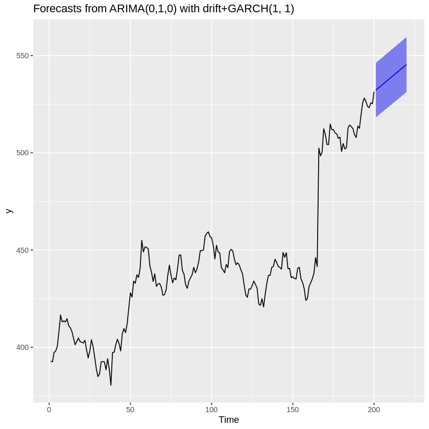
(res <- ahead::agnosticgarchf(fpp2::goog200,
                           FUN=forecast::auto.arima, h=20))

    Point Forecast    Lo 95    Hi 95
     532.1750 518.1879 546.1621
     532.8717 518.8757 546.8678
     533.5684 519.5635 547.5734
     534.2652 520.2513 548.2790
     534.9619 520.9391 548.9847
     535.6586 521.6269 549.6903
     536.3553 522.3148 550.3959
     537.0521 523.0026 551.1015
     537.7488 523.6905 551.8071
     538.4455 524.3783 552.5127
     539.1422 525.0662 553.2183
     539.8390 525.7540 553.9239
     540.5357 526.4419 554.6295
     541.2324 527.1298 555.3351
     541.9291 527.8176 556.0407
     542.6259 528.5055 556.7462
     543.3226 529.1934 557.4518
     544.0193 529.8813 558.1573
     544.7160 530.5692 558.8629
     545.4128 531.2571 559.5684

ggplot2::autoplot(res)

image-title-here

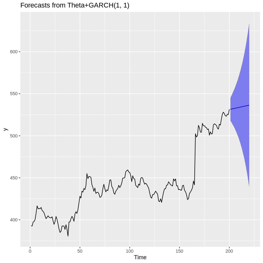
(res <- ahead::agnosticgarchf(fpp2::goog200,
                           FUN=forecast::thetaf, h=20))

    Point Forecast    Lo 95    Hi 95
     531.4982 518.2318 544.7646
     531.7610 516.1991 547.3230
     532.0238 514.1041 549.9436
     532.2867 511.9078 552.6655
     532.5495 509.5788 555.5201
     532.8123 507.0890 558.5356
     533.0751 504.4117 561.7384
     533.3379 501.5205 565.1553
     533.6007 498.3883 568.8131
     533.8635 494.9868 572.7402
     534.1263 491.2863 576.9663
     534.3891 487.2548 581.5234
     534.6519 482.8584 586.4454
     534.9147 478.0601 591.7693
     535.1775 472.8202 597.5348
     535.4403 467.0955 603.7851
     535.7031 460.8392 610.5670
     535.9659 454.0004 617.9315
     536.2288 446.5235 625.9340
     536.4916 438.3483 634.6349

ggplot2::autoplot(res)

image-title-here

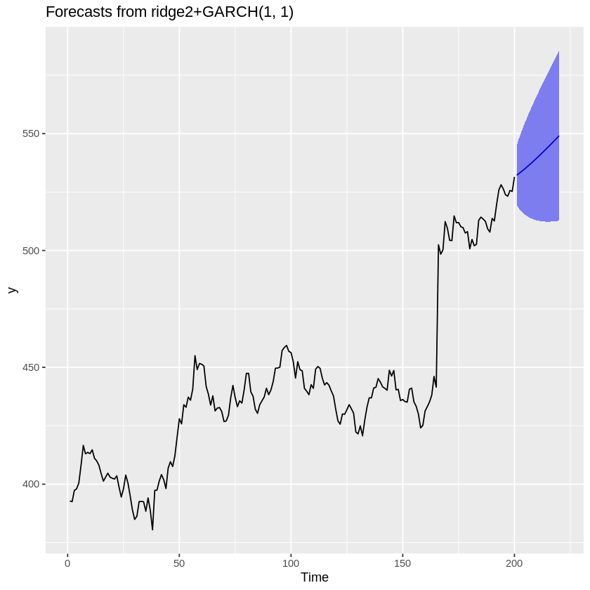
(res <- ahead::agnosticgarchf(fpp2::goog200,
                           FUN=ahead::ridge2f, h=20))

    Point Forecast    Lo 95    Hi 95
     532.1740 519.4742 544.8737
     532.9003 517.9900 547.8106
     533.6547 516.8217 550.4877
     534.4346 515.8770 552.9921
     535.2377 515.1028 555.3726
     536.0622 514.4648 557.6596
     536.9062 513.9392 559.8731
     537.7679 513.5087 562.0272
     538.6460 513.1598 564.1321
     539.5390 512.8824 566.1956
     540.4458 512.6679 568.2236
     541.3651 512.5096 570.2207
     542.2961 512.4018 572.1905
     543.2378 512.3395 574.1361
     544.1894 512.3188 576.0601
     545.1501 512.3359 577.9643
     546.1193 512.3879 579.8506
     547.0963 512.4721 581.7205
     548.0805 512.5859 583.5751
     549.0716 512.7274 585.4158

ggplot2::autoplot(res)

image-title-here

(res <- ahead::agnosticgarchf(fpp2::goog200,
                           FUN=ahead::loessf, h=20))

    Point Forecast    Lo 95    Hi 95
     544.3276 520.1558 568.4994
     548.2888 523.7199 572.8578
     552.0027 527.0698 576.9356
     554.1810 528.9140 579.4481
     556.8539 531.2797 582.4282
     560.3601 534.5032 586.2171
     561.5067 535.3893 587.6240
     565.6928 539.3353 592.0502
     567.2796 540.7006 593.8586
     570.1362 543.3525 596.9198
     574.0123 547.0395 600.9850
     578.5510 551.4034 605.6986
     580.8285 553.5191 608.1379
     584.2104 556.7512 611.6695
     587.9165 560.3187 615.5144
     591.1329 563.4066 618.8593
     594.0383 566.1929 621.8837
     595.6430 567.6872 623.5988
     602.2172 574.1590 630.2754
     604.7474 576.5943 632.9006

ggplot2::autoplot(res)

image-title-here

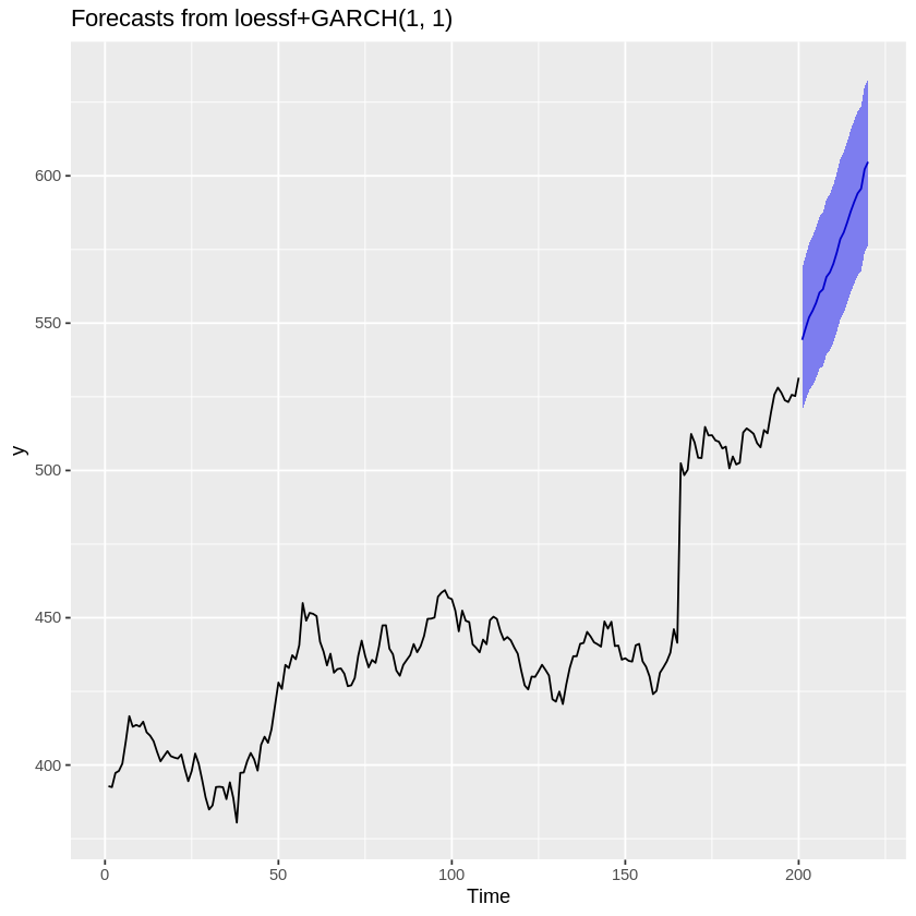
As we can see from the plots, combining any model with GARCH(1,1) provides a comprehensive view of both the expected stock prices and the associated uncertainty. This method is particularly useful for financial forecasting, where volatility plays a significant role.

Comments powered by Talkyard.

@misc{ tmoudiki20250923, author = { T. Moudiki }, title = { Combining any model with GARCH(1,1) for probabilistic stock forecasting }, url = { https://thierrymoudiki.github.io/blog/2025/09/23/r/ANYMODEL-plus-GARCH }, year = { 2025 } }