Update 2026-03-13: ARIMA is only used as a filter to remove the risk premium from the physical paths. It is not used to price the options.
In quantitative finance, pricing derivatives often requires working under a risk-neutral measure (Q) rather than the real-world physical measure (P). While the Girsanov theorem provides a theoretical framework for this change of measure, practical implementation can be challenging—especially for complex models like stochastic volatility with jumps (SVJD).
This blog post demonstrates a semi-parametric approach that bridges classical time series modeling with risk-neutral pricing. We’ll show how to:
- Simulate stock price paths under three different models (GBM, SVJD, Heston) using the physical measure
- Extract the risk premium using ARIMA modeling
- Transform physical paths to risk-neutral paths through residual resampling
- Price European options under the risk-neutral measure
Models Compared
- Geometric Brownian Motion (GBM): The classic Black-Scholes model with constant volatility
- Stochastic Volatility Jump Diffusion (SVJD): Incorporates both stochastic volatility and price jumps
- Heston Model: Stochastic volatility without jumps (a special case of SVJD)
Methodological Approach
Our semi-parametric method involves:
- Physical Simulation: Generate paths under the real-world measure with expected return μ
- Risk Premium Extraction: Fit ARIMA models to discounted price increments to capture serial dependence
- Residual Resampling: Use Gaussian density estimation to resample centered ARIMA residuals
- Risk-Neutral Path Generation:
Combine fitted ARIMA models with resampled residualsGenerate new paths by cumulatively summing the resampled centered residuals (starting from S0), then multiply by e^(rt) to return to price space - Option Pricing: Compute option prices as discounted expected payoffs under Q
R Packages Used
- esgtoolkit: For financial simulations and risk-neutral transformations
- ahead: For time series forecasting and residual resampling
- forecast (
auto.arima): For automatic ARIMA model selection
The complete reproducible code is presented below, organized in logical sections from simulation to option pricing.
## ----setup, include=FALSE------------------------------------------------------
knitr::opts_chunk$set(echo = TRUE)
## ----1-simulate-SVJD, cache=TRUE-----------------------------------------------
# ARIMA-Black-Scholes: Semi-Parametric Risk-Neutral Pricing
# T. Moudiki
# 2025-03-13
library(esgtoolkit)
library(forecast)
library(ahead)
# =============================================================================
# 1 - SVJD SIMULATION (Physical Measure)
# =============================================================================
set.seed(123)
n <- 250L
h <- 5
freq <- "daily"
r <- 0.05
maturity <- 5
S0 <- 100
mu <- 0.08
sigma <- 0.04
# Simulate under physical measure with stochastic volatility and jumps
sim_GBM <- esgtoolkit::simdiff(n=n, horizon = h, frequency = freq, x0=S0, theta1 = mu, theta2 = sigma)
sim_SVJD <- esgtoolkit::rsvjd(n=n, r0=mu)
sim_Heston <- esgtoolkit::rsvjd(n=n, r0=mu,
lambda = 0,
mu_J = 0,
sigma_J = 0)
cat("Simulation dimensions:\n")
cat("Start:", start(sim_SVJD), "\n")
cat("End:", end(sim_SVJD), "\n")
cat("Paths:", ncol(sim_SVJD), "\n")
cat("Time steps:", nrow(sim_SVJD), "\n\n")
par(mfrow=c(1, 3))
# Plot historical (physical measure) paths
esgtoolkit::esgplotbands(sim_GBM, main="GBM Paths under the Physical Measure",
xlab="Time",
ylab="Stock prices")
esgtoolkit::esgplotbands(sim_SVJD, main="SVJD Paths under the Physical Measure",
xlab="Time",
ylab="Stock prices")
esgtoolkit::esgplotbands(sim_Heston, main="Heston Paths under the Physical Measure",
xlab="Time",
ylab="Stock prices")
# Summary statistics
cat("Physical measure statistics (GBM):\n")
terminal_prices_physical_GBM <- sim_GBM[nrow(sim_GBM), ]
cat("Mean terminal price:", mean(terminal_prices_physical_GBM), "\n")
cat("Std terminal price:", sd(terminal_prices_physical_GBM), "\n")
cat("Expected under P:", S0 * exp(mu * maturity), "\n\n")
cat("Physical measure statistics (SVJD):\n")
terminal_prices_physical_SVJD <- sim_SVJD[nrow(sim_SVJD), ]
cat("Mean terminal price:", mean(terminal_prices_physical_SVJD), "\n")
cat("Std terminal price:", sd(terminal_prices_physical_SVJD), "\n")
cat("Expected under P:", S0 * exp(mu * maturity), "\n\n")
cat("Physical measure statistics (Heston):\n")
terminal_prices_physical_Heston <- sim_Heston[nrow(sim_Heston), ]
cat("Mean terminal price:", mean(terminal_prices_physical_Heston), "\n")
cat("Std terminal price:", sd(terminal_prices_physical_Heston), "\n")
cat("Expected under P:", S0 * exp(mu * maturity), "\n\n")
## ----2-compute-discounted, cache=TRUE------------------------------------------
# =============================================================================
# 2 - COMPUTE DISCOUNTED PRICES (Transform to Martingale Domain)
# =============================================================================
discounted_prices_GBM <- esgtoolkit::esgdiscountfactor(r=r, X=sim_GBM)
discounted_prices_SVJD <- esgtoolkit::esgdiscountfactor(r=r, X=sim_SVJD)
discounted_prices_Heston <- esgtoolkit::esgdiscountfactor(r=r, X=sim_Heston)
martingale_diff_GBM <- discounted_prices_GBM - S0
martingale_diff_SVJD <- discounted_prices_SVJD - S0
martingale_diff_Heston <- discounted_prices_Heston - S0
cat("Martingale differences dimensions (GBM):", dim(martingale_diff_GBM), "\n")
cat("Mean martingale diff (should be ≠ 0 under P):\n")
print(t.test(rowMeans(martingale_diff_GBM)))
cat("\nMartingale differences dimensions (SVJD):", dim(martingale_diff_SVJD), "\n")
cat("Mean martingale diff (should be ≠ 0 under P):\n")
print(t.test(rowMeans(martingale_diff_SVJD)))
cat("\nMartingale differences dimensions (Heston):", dim(martingale_diff_Heston), "\n")
cat("Mean martingale diff (should be ≠ 0 under P):\n")
print(t.test(rowMeans(martingale_diff_Heston)))
# =============================================================================
# 3 - VISUALIZE RISK PREMIUM
# =============================================================================
par(mfrow=c(2,2))
matplot(discounted_prices_GBM, type='l', col=rgb(0,0,1,0.3),
main="Discounted Stock Prices (Physical Measure - GBM)",
ylab="exp(-rt) * S_t", xlab="Time step")
abline(h=S0, col='red', lwd=2, lty=2)
matplot(discounted_prices_SVJD, type='l', col=rgb(0,0,1,0.3),
main="Discounted Stock Prices (Physical Measure - SVJD)",
ylab="exp(-rt) * S_t", xlab="Time step")
abline(h=S0, col='red', lwd=2, lty=2)
matplot(discounted_prices_Heston, type='l', col=rgb(0,0,1,0.3),
main="Discounted Stock Prices (Physical Measure - Heston)",
ylab="exp(-rt) * S_t", xlab="Time step")
abline(h=S0, col='red', lwd=2, lty=2)
par(mfrow=c(1,1))
mean_disc_path_GBM <- rowMeans(discounted_prices_GBM)
times_plot <- as.numeric(time(discounted_prices_GBM))
plot(times_plot, mean_disc_path_GBM, type='l', lwd=2, col='blue',
main="Risk Premium in Discounted Prices (GBM)",
xlab="Time (years)", ylab="E[exp(-rt)*S_t]")
abline(h=S0, col='red', lwd=2, lty=2)
lines(times_plot, S0 * exp((mu-r)*times_plot), col='green', lwd=2, lty=3)
legend("topleft",
legend=c("Empirical mean", "S0", "Theoretical (μ-r drift)"),
col=c('blue','red','green'), lty=c(1,2,3), lwd=2)
mean_disc_path_SVJD <- rowMeans(discounted_prices_SVJD)
times_plot <- as.numeric(time(discounted_prices_SVJD))
plot(times_plot, mean_disc_path_SVJD, type='l', lwd=2, col='blue',
main="Risk Premium in Discounted Prices (SVJD)",
xlab="Time (years)", ylab="E[exp(-rt)*S_t]")
abline(h=S0, col='red', lwd=2, lty=2)
lines(times_plot, S0 * exp((mu-r)*times_plot), col='green', lwd=2, lty=3)
legend("topleft",
legend=c("Empirical mean", "S0", "Theoretical (μ-r drift)"),
col=c('blue','red','green'), lty=c(1,2,3), lwd=2)
mean_disc_path_Heston <- rowMeans(discounted_prices_Heston)
times_plot <- as.numeric(time(discounted_prices_Heston))
plot(times_plot, mean_disc_path_Heston, type='l', lwd=2, col='blue',
main="Risk Premium in Discounted Prices (Heston)",
xlab="Time (years)", ylab="E[exp(-rt)*S_t]")
abline(h=S0, col='red', lwd=2, lty=2)
lines(times_plot, S0 * exp((mu-r)*times_plot), col='green', lwd=2, lty=3)
legend("topleft",
legend=c("Empirical mean", "S0", "Theoretical (μ-r drift)"),
col=c('blue','red','green'), lty=c(1,2,3), lwd=2)
## ----3-fit-ARIMA, cache=TRUE, eval=TRUE----------------------------------------
# =============================================================================
# 4 - FIT ARIMA MODELS TO EXTRACT RISK PREMIUM
# =============================================================================
n_periods <- nrow(martingale_diff_GBM)
n_paths <- ncol(martingale_diff_GBM)
martingale_increments_GBM <- diff(martingale_diff_GBM)
martingale_increments_SVJD <- diff(martingale_diff_SVJD)
martingale_increments_Heston <- diff(martingale_diff_Heston)
# Initialize storage arrays
arima_residuals_GBM <- array(NA, dim = c(nrow(martingale_increments_GBM), n_paths))
centered_arima_residuals_GBM <- array(NA, dim = c(nrow(martingale_increments_GBM), n_paths))
means_arima_residuals_GBM <- rep(NA, n_paths)
arima_models_GBM <- list()
arima_residuals_SVJD <- array(NA, dim = c(nrow(martingale_increments_SVJD), n_paths))
centered_arima_residuals_SVJD <- array(NA, dim = c(nrow(martingale_increments_SVJD), n_paths))
means_arima_residuals_SVJD <- rep(NA, n_paths)
arima_models_SVJD <- list()
arima_residuals_Heston <- array(NA, dim = c(nrow(martingale_increments_Heston), n_paths))
centered_arima_residuals_Heston <- array(NA, dim = c(nrow(martingale_increments_Heston), n_paths))
means_arima_residuals_Heston <- rep(NA, n_paths)
arima_models_Heston <- list()
# Fit ARIMA models to GBM
cat("Fitting ARIMA models to", n_paths, "GBM paths...\n")
for (i in 1:n_paths) {
y <- as.numeric(martingale_increments_GBM[, i])
fit <- forecast::auto.arima(y, allowmean = FALSE)
arima_models_GBM[[i]] <- fit
res <- as.numeric(residuals(fit))
arima_residuals_GBM[, i] <- res
centre_arima_residuals <- scale(res, center = TRUE, scale = FALSE)
means_arima_residuals_GBM[i] <- attr(centre_arima_residuals, "scaled:center")
centered_arima_residuals_GBM[, i] <- centre_arima_residuals[,1]
}
# Fit ARIMA models to SVJD
cat("Fitting ARIMA models to", n_paths, "SVJD paths...\n")
for (i in 1:n_paths) {
y <- as.numeric(martingale_increments_SVJD[, i])
fit <- forecast::auto.arima(y, allowmean = FALSE)
arima_models_SVJD[[i]] <- fit
res <- as.numeric(residuals(fit))
arima_residuals_SVJD[, i] <- res
centre_arima_residuals <- scale(res, center = TRUE, scale = FALSE)
means_arima_residuals_SVJD[i] <- attr(centre_arima_residuals, "scaled:center")
centered_arima_residuals_SVJD[, i] <- centre_arima_residuals[,1]
}
# Fit ARIMA models to Heston
cat("Fitting ARIMA models to", n_paths, "Heston paths...\n")
for (i in 1:n_paths) {
y <- as.numeric(martingale_increments_Heston[, i])
fit <- forecast::auto.arima(y, allowmean = FALSE)
arima_models_Heston[[i]] <- fit
res <- as.numeric(residuals(fit))
arima_residuals_Heston[, i] <- res
centre_arima_residuals <- scale(res, center = TRUE, scale = FALSE)
means_arima_residuals_Heston[i] <- attr(centre_arima_residuals, "scaled:center")
centered_arima_residuals_Heston[, i] <- centre_arima_residuals[,1]
}
cat("\nARIMA model summary (first 5 GBM paths):\n")
for (i in 1:min(5, n_paths)) {
cat("Path", i, ":", as.character(arima_models_GBM[[i]]), "\n")
}
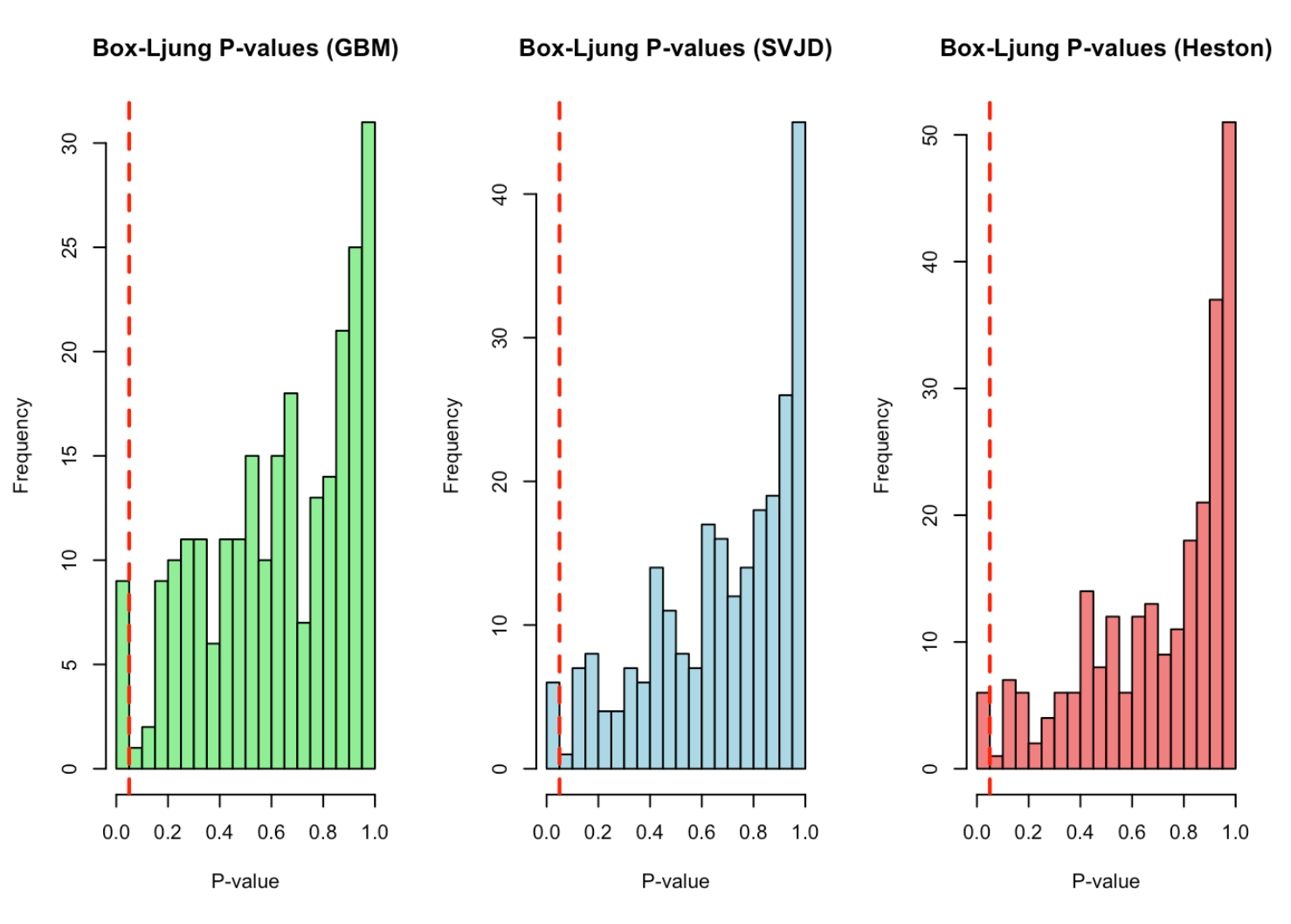
# Box-Ljung tests
pvalues_GBM <- sapply(1:ncol(centered_arima_residuals_GBM),
function(i) Box.test(centered_arima_residuals_GBM[,i])$p.value)
cat("\nBox-Ljung test p-values (GBM):\n")
cat("Mean p-value:", mean(pvalues_GBM), "\n")
cat("Proportion > 0.05:", mean(pvalues_GBM > 0.05), "\n")
pvalues_SVJD <- sapply(1:ncol(centered_arima_residuals_SVJD),
function(i) Box.test(centered_arima_residuals_SVJD[,i])$p.value)
cat("\nBox-Ljung test p-values (SVJD):\n")
cat("Mean p-value:", mean(pvalues_SVJD), "\n")
cat("Proportion > 0.05:", mean(pvalues_SVJD > 0.05), "\n")
pvalues_Heston <- sapply(1:ncol(centered_arima_residuals_Heston),
function(i) Box.test(centered_arima_residuals_Heston[,i])$p.value)
cat("\nBox-Ljung test p-values (Heston):\n")
cat("Mean p-value:", mean(pvalues_Heston), "\n")
cat("Proportion > 0.05:", mean(pvalues_Heston > 0.05), "\n")
par(mfrow=c(1,3))
hist(pvalues_GBM, breaks=20, col='lightgreen',
main="Box-Ljung P-values (GBM)",
xlab="P-value")
abline(v=0.05, col='red', lwd=2, lty=2)
hist(pvalues_SVJD, breaks=20, col='lightblue',
main="Box-Ljung P-values (SVJD)",
xlab="P-value")
abline(v=0.05, col='red', lwd=2, lty=2)
hist(pvalues_Heston, breaks=20, col='lightcoral',
main="Box-Ljung P-values (Heston)",
xlab="P-value")
abline(v=0.05, col='red', lwd=2, lty=2)
par(mfrow=c(1,1))
## ----4-generate-rn-paths, cache=TRUE, eval=TRUE--------------------------------
# =============================================================================
# 5 - GENERATE RISK-NEUTRAL PATHS
# =============================================================================
cat("\n\nGenerating risk-neutral paths from ALL historical paths...\n")
n_sim_per_path <- 20 # Generate 10 paths per historical path
times <- seq(0, maturity, length.out = n_periods)
discount_factor <- exp(r * times)
# Storage for all risk-neutral paths
all_S_tilde_GBM <- list()
all_S_tilde_SVJD <- list()
all_S_tilde_Heston <- list()
# Generate GBM risk-neutral paths
for (i in 1:n_paths) {
resampled_residuals <- ahead::rgaussiandens(centered_arima_residuals_GBM[, i],
p = n_sim_per_path)
fit <- arima_models_GBM[[i]]
fitted_increments <- as.numeric(fitted(fit))
discounted_path <- matrix(0, nrow = n_periods, ncol = n_sim_per_path)
discounted_path[1, ] <- S0
increments <- resampled_residuals[1:(n_periods - 1), ]
discounted_path[-1, ] <- S0 + apply(increments, 2, cumsum)
S_tilde_price <- discounted_path * discount_factor
all_S_tilde_GBM[[i]] <- S_tilde_price
}
# Generate SVJD risk-neutral paths
for (i in 1:n_paths) {
resampled_residuals <- ahead::rgaussiandens(centered_arima_residuals_SVJD[, i],
p = n_sim_per_path)
fit <- arima_models_SVJD[[i]]
fitted_increments <- as.numeric(fitted(fit))
discounted_path <- matrix(0, nrow = n_periods, ncol = n_sim_per_path)
discounted_path[1, ] <- S0
increments <- resampled_residuals[1:(n_periods - 1), ]
discounted_path[-1, ] <- S0 + apply(increments, 2, cumsum)
S_tilde_price <- discounted_path * discount_factor
all_S_tilde_SVJD[[i]] <- S_tilde_price
}
# Generate Heston risk-neutral paths
for (i in 1:n_paths) {
resampled_residuals <- ahead::rgaussiandens(centered_arima_residuals_Heston[, i],
p = n_sim_per_path)
fit <- arima_models_Heston[[i]]
fitted_increments <- as.numeric(fitted(fit))
discounted_path <- matrix(0, nrow = n_periods, ncol = n_sim_per_path)
discounted_path[1, ] <- S0
increments <- resampled_residuals[1:(n_periods - 1), ]
discounted_path[-1, ] <- S0 + apply(increments, 2, cumsum)
S_tilde_price <- discounted_path * discount_factor
all_S_tilde_Heston[[i]] <- S_tilde_price
}
# Combine all paths
S_tilde_combined_GBM <- do.call(cbind, all_S_tilde_GBM)
cat("Total GBM risk-neutral paths generated:", ncol(S_tilde_combined_GBM), "\n")
S_tilde_combined_SVJD <- do.call(cbind, all_S_tilde_SVJD)
cat("Total SVJD risk-neutral paths generated:", ncol(S_tilde_combined_SVJD), "\n")
S_tilde_combined_Heston <- do.call(cbind, all_S_tilde_Heston)
cat("Total Heston risk-neutral paths generated:", ncol(S_tilde_combined_Heston), "\n\n")
# Convert to time series
S_tilde_ts_GBM <- ts(S_tilde_combined_GBM, start = start(sim_GBM),
frequency = frequency(sim_GBM))
S_tilde_ts_SVJD <- ts(S_tilde_combined_SVJD, start = start(sim_SVJD),
frequency = frequency(sim_SVJD))
S_tilde_ts_Heston <- ts(S_tilde_combined_Heston, start = start(sim_Heston),
frequency = frequency(sim_Heston))
# Visualize risk-neutral paths
par(mfrow=c(1,3))
esgtoolkit::esgplotbands(S_tilde_ts_GBM,
main="Risk-Neutral Paths - GBM")
esgtoolkit::esgplotbands(S_tilde_ts_SVJD,
main="Risk-Neutral Paths - SVJD")
esgtoolkit::esgplotbands(S_tilde_ts_Heston,
main="Risk-Neutral Paths - Heston")
# Sample plots
par(mfrow=c(1,3))
matplot(S_tilde_combined_GBM[, sample(ncol(S_tilde_combined_GBM), 200)],
type='l', col=rgb(0,0,1,0.1),
main="Risk-Neutral Paths (GBM)",
xlab="Time step", ylab="Stock Price")
lines(rowMeans(S_tilde_combined_GBM), col='red', lwd=3)
abline(h=S0, col='green', lwd=2, lty=2)
matplot(S_tilde_combined_SVJD[, sample(ncol(S_tilde_combined_SVJD), 200)],
type='l', col=rgb(0,0,1,0.1),
main="Risk-Neutral Paths (SVJD)",
xlab="Time step", ylab="Stock Price")
lines(rowMeans(S_tilde_combined_SVJD), col='red', lwd=3)
abline(h=S0, col='green', lwd=2, lty=2)
matplot(S_tilde_combined_Heston[, sample(ncol(S_tilde_combined_Heston), 200)],
type='l', col=rgb(0,0,1,0.1),
main="Risk-Neutral Paths (Heston)",
xlab="Time step", ylab="Stock Price")
lines(rowMeans(S_tilde_combined_Heston), col='red', lwd=3)
abline(h=S0, col='green', lwd=2, lty=2)
par(mfrow=c(1,1))
## ----5-rn-verif, cache=TRUE, eval=TRUE-----------------------------------------
# =============================================================================
# 6 - VERIFY RISK-NEUTRAL PROPERTY
# =============================================================================
cat("\n=== RISK-NEUTRAL VERIFICATION ===\n\n")
terminal_prices_rn_GBM <- S_tilde_combined_GBM[n_periods, ]
terminal_prices_rn_SVJD <- S_tilde_combined_SVJD[n_periods, ]
terminal_prices_rn_Heston <- S_tilde_combined_Heston[n_periods, ]
capitalized_stock_price <- S0 * exp(r * maturity)
cat("GBM Risk-Neutral Verification:\n")
cat("Expected terminal price (Q):", capitalized_stock_price, "\n")
cat("Empirical mean:", mean(terminal_prices_rn_GBM), "\n")
cat("Difference:", mean(terminal_prices_rn_GBM) - capitalized_stock_price, "\n")
print(t.test(terminal_prices_rn_GBM - capitalized_stock_price))
cat("\nSVJD Risk-Neutral Verification:\n")
cat("Expected terminal price (Q):", capitalized_stock_price, "\n")
cat("Empirical mean:", mean(terminal_prices_rn_SVJD), "\n")
cat("Difference:", mean(terminal_prices_rn_SVJD) - capitalized_stock_price, "\n")
print(t.test(terminal_prices_rn_SVJD - capitalized_stock_price))
cat("\nHeston Risk-Neutral Verification:\n")
cat("Expected terminal price (Q):", capitalized_stock_price, "\n")
cat("Empirical mean:", mean(terminal_prices_rn_Heston), "\n")
cat("Difference:", mean(terminal_prices_rn_Heston) - capitalized_stock_price, "\n")
print(t.test(terminal_prices_rn_Heston - capitalized_stock_price))
# Visualization comparison
par(mfrow=c(3, 2))
hist(terminal_prices_physical_GBM, breaks=30, col=rgb(1,0,0,0.5),
main="Terminal Prices: Physical (GBM)",
xlab="Price", xlim=c(50, 300))
abline(v=mean(terminal_prices_physical_GBM), col='red', lwd=2)
abline(v=S0*exp(mu*maturity), col='blue', lwd=2, lty=2)
hist(terminal_prices_rn_GBM, breaks=30, col=rgb(0,0,1,0.5),
main="Terminal Prices: Risk-Neutral (GBM)",
xlab="Price", xlim=c(50, 300))
abline(v=mean(terminal_prices_rn_GBM), col='blue', lwd=2)
abline(v=S0*exp(r*maturity), col='red', lwd=2, lty=2)
hist(terminal_prices_physical_SVJD, breaks=30, col=rgb(1,0,0,0.5),
main="Terminal Prices: Physical (SVJD)",
xlab="Price", xlim=c(50, 300))
abline(v=mean(terminal_prices_physical_SVJD), col='red', lwd=2)
abline(v=S0*exp(mu*maturity), col='blue', lwd=2, lty=2)
hist(terminal_prices_rn_SVJD, breaks=30, col=rgb(0,0,1,0.5),
main="Terminal Prices: Risk-Neutral (SVJD)",
xlab="Price", xlim=c(50, 300))
abline(v=mean(terminal_prices_rn_SVJD), col='blue', lwd=2)
abline(v=S0*exp(r*maturity), col='red', lwd=2, lty=2)
hist(terminal_prices_physical_Heston, breaks=30, col=rgb(1,0,0,0.5),
main="Terminal Prices: Physical (Heston)",
xlab="Price", xlim=c(50, 300))
abline(v=mean(terminal_prices_physical_Heston), col='red', lwd=2)
abline(v=S0*exp(mu*maturity), col='blue', lwd=2, lty=2)
hist(terminal_prices_rn_Heston, breaks=30, col=rgb(0,0,1,0.5),
main="Terminal Prices: Risk-Neutral (Heston)",
xlab="Price", xlim=c(50, 300))
abline(v=mean(terminal_prices_rn_Heston), col='blue', lwd=2)
abline(v=S0*exp(r*maturity), col='red', lwd=2, lty=2)
par(mfrow=c(1,1))
## ----6-option-pricing, cache=TRUE, eval=TRUE-----------------------------------
# =============================================================================
# 7 - OPTION PRICING
# =============================================================================
cat("\n=== OPTION PRICING ===\n\n")
bs_price <- function(S, K, r, sigma, T, q = 0) {
d1 <- (log(S / K) + (r - q + 0.5 * sigma^2) * T) / (sigma * sqrt(T))
d2 <- d1 - sigma * sqrt(T)
call <- S * exp(-q * T) * pnorm(d1) - K * exp(-r * T) * pnorm(d2)
put <- K * exp(-r * T) * pnorm(-d2) - S * exp(-q * T) * pnorm(-d1)
list(call = call, put = put)
}
strikes <- seq(80, 160, by=10)
d_f <- exp(-r * maturity)
# Function to price options
price_options <- function(terminal_prices, strikes, discount_factor) {
n_strikes <- length(strikes)
call_prices <- numeric(n_strikes)
bs_call_prices <- numeric(n_strikes)
put_prices <- numeric(n_strikes)
bs_put_prices <- numeric(n_strikes)
call_se <- numeric(n_strikes)
put_se <- numeric(n_strikes)
for (k in 1:n_strikes) {
K <- strikes[k]
call_payoffs <- pmax(terminal_prices - K, 0)
call_prices[k] <- mean(call_payoffs) * discount_factor
call_se[k] <- sd(call_payoffs) / sqrt(length(call_payoffs)) * discount_factor
put_payoffs <- pmax(K - terminal_prices, 0)
put_prices[k] <- mean(put_payoffs) * discount_factor
put_se[k] <- sd(put_payoffs) / sqrt(length(put_payoffs)) * discount_factor
bs_prices <- bs_price(S0, K, r, sigma=sigma, T=5, q = 0)
bs_call_prices[k] <- bs_prices$call
bs_put_prices[k] <- bs_prices$put
}
list(call_prices = call_prices, put_prices = put_prices,
bs_call_prices = bs_call_prices, bs_put_prices = bs_put_prices,
call_se = call_se, put_se = put_se)
}
# Price options for all models
options_GBM <- price_options(terminal_prices_rn_GBM, strikes, d_f)
options_SVJD <- price_options(terminal_prices_rn_SVJD, strikes, d_f)
options_Heston <- price_options(terminal_prices_rn_Heston, strikes, d_f)
## ------------------------------------------------------------------------------
kableExtra::kable(as.data.frame(options_GBM))
kableExtra::kable(as.data.frame(options_Heston))
kableExtra::kable(as.data.frame(options_SVJD))
Full code and additional details are available on GitHub:
https://github.com/thierrymoudiki/2025-12-07-risk-neutralization-with-ARIMA
The preprint of the associated research paper can be found here:
PS: It’s worth mentioning that this approach can produce negative prices
For attribution, please cite this work as:
T. Moudiki (2025-12-07). ARIMA Pricing: Semi-Parametric Market price of risk for Risk-Neutral Pricing (code + preprint). Retrieved from https://thierrymoudiki.github.io/blog/2025/12/07/r/forecasting/ARIMA-Pricing
BibTeX citation (remove empty spaces)
        @misc{ tmoudiki20251207,
          author = { T. Moudiki },
          title = { ARIMA Pricing: Semi-Parametric Market price of risk for Risk-Neutral Pricing (code + preprint) },
          url = { https://thierrymoudiki.github.io/blog/2025/12/07/r/forecasting/ARIMA-Pricing },
          year = { 2025 } }

Previous publications
- My last R posts: How conformalization helps weak models, fast conformal prediction with jackknife+ (and no refitting), and sklearn in R Jul 13, 2026
- Natively Interpretable Boosting Jul 12, 2026
- Fast conformal prediction (no refitting) for some Machine Learning models via closed-form jackknife plus Jun 27, 2026
- Using scikit-learn models in R easily with the tisthemachinelearner package Jun 21, 2026
- No-Code Machine Learning in Excel with the Techtonique API Jun 14, 2026
- How Conformal Prediction Makes Linear Models Good Enough — An Example Using R Package mlS3 Jun 7, 2026
- Techtonique dot net, the Machine Learning web API, is back online (but more like a passion project for now) May 31, 2026
- Conformalized TabICL: Prediction Intervals for a State-Of-The-Art Tabular Foundation Model in Python and R May 21, 2026
- Conformalized TabPFN: Prediction Intervals for a Pretrained Transformer for Tabular Data in Python and R May 17, 2026
- Probabilistic Time Series Cross-Validation with R package crossvalidation May 16, 2026
- One interface, (Almost) Every Classifier (and Regressor): unifiedml v0.3.0 May 9, 2026
- You Don't Need to Learn All the Weights on tabular data: The Case for rvflnet (a nonlinear expressive glmnet) on regression, classification and survival analysis May 2, 2026
- Survival analysis with sklearn, glmnet, keras, pytorch, lightgbm, xgboost, nnetsauce, mlsauce Part 2 Apr 28, 2026
- Any Sklearn Regressor as a Survival Model — Does It Actually Work? Benchmarking vs Established Packages Apr 26, 2026
- Conformal Optimization Beats Bayesian Optimization, Optuna and Random Search on 72 classification Datasets Apr 19, 2026
- `mlS3` — A Unified S3 Machine Learning Interface in R Apr 12, 2026
- One interface, (Almost) Every Classifier: unifiedml v0.2.1 Apr 4, 2026
- Techtonique dot net is down until further notice Apr 1, 2026
- Explaining Time-Series Forecasts with Sensitivity Analysis (ahead::dynrmf and external regressors) Mar 29, 2026
- Python version of 'Option pricing using time series models as market price of risk Pt.3' Mar 22, 2026
- Option pricing using time series models as market price of risk Pt.3 Mar 16, 2026
- Explaining Time-Series Forecasts with Exact Shapley Values (ahead::dynrmf with external regressors applied to scenarios) Mar 8, 2026
- My Presentation at Risk 2026: Lightweight Transfer Learning for Financial Forecasting Mar 1, 2026
- nnetsauce with and without jax for GPU acceleration Feb 23, 2026
- Understanding Boosted Configuration Networks (combined neural networks and boosting): An Intuitive Guide Through Their Hyperparameters Feb 16, 2026
- R version of Python package survivalist, for model-agnostic survival analysis Feb 9, 2026
- Presenting Lightweight Transfer Learning for Financial Forecasting (Risk 2026) Feb 4, 2026
- Option pricing using time series models as market price of risk Feb 1, 2026
- Enhancing Time Series Forecasting (ahead::ridge2f) with Attention-Based Context Vectors (ahead::contextridge2f) Jan 31, 2026
- Overfitting and scaling (on GPU T4) tests on nnetsauce.CustomRegressor Jan 29, 2026
- Beyond Cross-validation: Hyperparameter Optimization via Generalization Gap Modeling Jan 25, 2026
- GPopt for Machine Learning (hyperparameters' tuning) Jan 21, 2026
- rtopy: an R to Python bridge -- novelties Jan 8, 2026
- Python examples for 'Beyond Nelson-Siegel and splines: A model- agnostic Machine Learning framework for discount curve calibration, interpolation and extrapolation' Jan 3, 2026
- Forecasting benchmark: Dynrmf (a new serious competitor in town) vs Theta Method on M-Competitions and Tourism competitition Jan 1, 2026
- Finally figured out a way to port python packages to R using uv and reticulate: example with nnetsauce Dec 17, 2025
- Overfitting Random Fourier Features: Universal Approximation Property Dec 13, 2025
- Counterfactual Scenario Analysis with ahead::ridge2f Dec 11, 2025
- Zero-Shot Probabilistic Time Series Forecasting with TabPFN 2.5 and nnetsauce Dec 10, 2025
- ARIMA Pricing: Semi-Parametric Market price of risk for Risk-Neutral Pricing (code + preprint) Dec 7, 2025
- Analyzing Paper Reviews with LLMs: I Used ChatGPT, DeepSeek, Qwen, Mistral, Gemini, and Claude (and you should too + publish the analysis) Dec 3, 2025
- tisthemachinelearner: New Workflow with uv for R Integration of scikit-learn Dec 1, 2025
- (ICYMI) RPweave: Unified R + Python + LaTeX System using uv Nov 21, 2025
- unifiedml: A Unified Machine Learning Interface for R, is now on CRAN + Discussion about AI replacing humans Nov 16, 2025
- Context-aware Theta forecasting Method: Extending Classical Time Series Forecasting with Machine Learning Nov 13, 2025
- unifiedml in R: A Unified Machine Learning Interface Nov 5, 2025
- Deterministic Shift Adjustment in Arbitrage-Free Pricing (historical to risk-neutral short rates) Oct 28, 2025
- New instantaneous short rates models with their deterministic shift adjustment, for historical and risk-neutral simulation Oct 27, 2025
- RPweave: Unified R + Python + LaTeX System using uv Oct 19, 2025
- GAN-like Synthetic Data Generation Examples (on univariate, multivariate distributions, digits recognition, Fashion-MNIST, stock returns, and Olivetti faces) with DistroSimulator Oct 19, 2025
- R port of llama2.c Oct 9, 2025
- Native uncertainty quantification for time series with NGBoost Oct 8, 2025
- NGBoost (Natural Gradient Boosting) for Regression, Classification, Time Series forecasting and Reserving Oct 6, 2025
- Real-time pricing with a pretrained probabilistic stock return model Oct 1, 2025
- Combining any model with GARCH(1,1) for probabilistic stock forecasting Sep 23, 2025
- Generating Synthetic Data with R-vine Copulas using esgtoolkit in R Sep 21, 2025
- Reimagining Equity Solvency Capital Requirement Approximation (one of my Master's Thesis subjects): From Bilinear Interpolation to Probabilistic Machine Learning Sep 16, 2025
- Transfer Learning using ahead::ridge2f on synthetic stocks returns Pt.2: synthetic data generation Sep 9, 2025
- Transfer Learning using ahead::ridge2f on synthetic stocks returns Sep 8, 2025
- I'm supposed to present 'Conformal Predictive Simulations for Univariate Time Series' at COPA CONFERENCE 2025 in London... Sep 4, 2025
- external regressors in ahead::dynrmf's interface for Machine learning forecasting Sep 1, 2025
- Another interesting decision, now for 'Beyond Nelson-Siegel and splines: A model-agnostic Machine Learning framework for discount curve calibration, interpolation and extrapolation' Aug 20, 2025
- Boosting any randomized based learner for regression, classification and univariate/multivariate time series forcasting Jul 26, 2025
- New nnetsauce version with CustomBackPropRegressor (CustomRegressor with Backpropagation) and ElasticNet2Regressor (Ridge2 with ElasticNet regularization) Jul 15, 2025
- mlsauce (home to a model-agnostic gradient boosting algorithm) can now be installed from PyPI. Jul 10, 2025
- A user-friendly graphical interface to techtonique dot net's API (will eventually contain graphics). Jul 8, 2025
- Calling =TECHTO_MLCLASSIFICATION for Machine Learning supervised CLASSIFICATION in Excel is just a matter of copying and pasting Jul 7, 2025
- Calling =TECHTO_MLREGRESSION for Machine Learning supervised regression in Excel is just a matter of copying and pasting Jul 6, 2025
- Calling =TECHTO_RESERVING and =TECHTO_MLRESERVING for claims triangle reserving in Excel is just a matter of copying and pasting Jul 5, 2025
- Calling =TECHTO_SURVIVAL for Survival Analysis in Excel is just a matter of copying and pasting Jul 4, 2025
- Calling =TECHTO_SIMULATION for Stochastic Simulation in Excel is just a matter of copying and pasting Jul 3, 2025
- Calling =TECHTO_FORECAST for forecasting in Excel is just a matter of copying and pasting Jul 2, 2025
- Random Vector Functional Link (RVFL) artificial neural network with 2 regularization parameters successfully used for forecasting/synthetic simulation in professional settings: Extensions (including Bayesian) Jul 1, 2025
- R version of 'Backpropagating quasi-randomized neural networks' Jun 24, 2025
- Backpropagating quasi-randomized neural networks Jun 23, 2025
- Beyond ARMA-GARCH: leveraging any statistical model for volatility forecasting Jun 21, 2025
- Stacked generalization (Machine Learning model stacking) + conformal prediction for forecasting with ahead::mlf Jun 18, 2025
- An Overfitting dilemma: XGBoost Default Hyperparameters vs GenericBooster + LinearRegression Default Hyperparameters Jun 14, 2025
- Programming language-agnostic reserving using RidgeCV, LightGBM, XGBoost, and ExtraTrees Machine Learning models Jun 13, 2025
- Free R, Python and SQL editors in techtonique dot net Jun 9, 2025
- Beyond Nelson-Siegel and splines: A model-agnostic Machine Learning framework for discount curve calibration, interpolation and extrapolation Jun 7, 2025
- scikit-learn, glmnet, xgboost, lightgbm, pytorch, keras, nnetsauce in probabilistic Machine Learning (for longitudinal data) Reserving (work in progress) Jun 6, 2025
- R version of Probabilistic Machine Learning (for longitudinal data) Reserving (work in progress) Jun 5, 2025
- Probabilistic Machine Learning (for longitudinal data) Reserving (work in progress) Jun 4, 2025
- Python version of Beyond ARMA-GARCH: leveraging model-agnostic Quasi-Randomized networks and conformal prediction for nonparametric probabilistic stock forecasting (ML-ARCH) Jun 3, 2025
- Beyond ARMA-GARCH: leveraging model-agnostic Machine Learning and conformal prediction for nonparametric probabilistic stock forecasting (ML-ARCH) Jun 2, 2025
- Permutations and SHAPley values for feature importance in techtonique dot net's API (with R + Python + the command line) Jun 1, 2025
- Which patient is going to survive longer? Another guide to using techtonique dot net's API (with R + Python + the command line) for survival analysis May 31, 2025
- A Guide to Using techtonique.net's API and rush for simulating and plotting Stochastic Scenarios May 30, 2025
- Simulating Stochastic Scenarios with Diffusion Models: A Guide to Using techtonique.net's API for the purpose May 29, 2025
- Will my apartment in 5th avenue be overpriced or not? Harnessing the power of www.techtonique.net (+ xgboost, lightgbm, catboost) to find out May 28, 2025
- How long must I wait until something happens: A Comprehensive Guide to Survival Analysis via an API May 27, 2025
- Harnessing the Power of techtonique.net: A Comprehensive Guide to Machine Learning Classification via an API May 26, 2025
- Quantile regression with any regressor -- Examples with RandomForestRegressor, RidgeCV, KNeighborsRegressor May 20, 2025
- Survival stacking: survival analysis translated as supervised classification in R and Python May 5, 2025
- 'Bayesian' optimization of hyperparameters in a R machine learning model using the bayesianrvfl package Apr 25, 2025
- A lightweight interface to scikit-learn in R: Bayesian and Conformal prediction Apr 21, 2025
- A lightweight interface to scikit-learn in R Pt.2: probabilistic time series forecasting in conjunction with ahead::dynrmf Apr 20, 2025
- Extending the Theta forecasting method to GLMs, GAMs, GLMBOOST and attention: benchmarking on Tourism, M1, M3 and M4 competition data sets (28000 series) Apr 14, 2025
- Extending the Theta forecasting method to GLMs and attention Apr 8, 2025
- Nonlinear conformalized Generalized Linear Models (GLMs) with R package 'rvfl' (and other models) Mar 31, 2025
- Probabilistic Time Series Forecasting (predictive simulations) in Microsoft Excel using Python, xlwings lite and www.techtonique.net Mar 28, 2025
- Conformalize (improved prediction intervals and simulations) any R Machine Learning model with misc::conformalize Mar 25, 2025
- My poster for the 18th FINANCIAL RISKS INTERNATIONAL FORUM by Institut Louis Bachelier/Fondation du Risque/Europlace Institute of Finance Mar 19, 2025
- Interpretable probabilistic kernel ridge regression using Matérn 3/2 kernels Mar 16, 2025
- (News from) Probabilistic Forecasting of univariate and multivariate Time Series using Quasi-Randomized Neural Networks (Ridge2) and Conformal Prediction Mar 9, 2025
- Word-Online: re-creating Karpathy's char-RNN (with supervised linear online learning of word embeddings) for text completion Mar 8, 2025
- CRAN-like repository for most recent releases of Techtonique's R packages Mar 2, 2025
- Presenting 'Online Probabilistic Estimation of Carbon Beta and Carbon Shapley Values for Financial and Climate Risk' at Institut Louis Bachelier Feb 27, 2025
- Web app with DeepSeek R1 and Hugging Face API for chatting Feb 23, 2025
- tisthemachinelearner: A Lightweight interface to scikit-learn with 2 classes, Classifier and Regressor (in Python and R) Feb 17, 2025
- R version of survivalist: Probabilistic model-agnostic survival analysis using scikit-learn, xgboost, lightgbm (and conformal prediction) Feb 12, 2025
- Model-agnostic global Survival Prediction of Patients with Myeloid Leukemia in QRT/Gustave Roussy Challenge (challengedata.ens.fr): Python's survivalist Quickstart Feb 10, 2025
- A simple test of the martingale hypothesis in esgtoolkit Feb 3, 2025
- Command Line Interface (CLI) for techtonique.net's API Jan 31, 2025
- Gradient-Boosting and Boostrap aggregating anything (alert: high performance): Part5, easier install and Rust backend Jan 27, 2025
- Just got a paper on conformal prediction REJECTED by International Journal of Forecasting despite evidence on 30,000 time series (and more). What's going on? Part2: 1311 time series from the Tourism competition Jan 20, 2025
- Techtonique is released! (with a tutorial in various programming languages and formats) Jan 14, 2025
- Univariate and Multivariate Probabilistic Forecasting with nnetsauce and TabPFN Jan 14, 2025
- Just got a paper on conformal prediction REJECTED by International Journal of Forecasting despite evidence on 30,000 time series (and more). What's going on? Jan 5, 2025
- Python and Interactive dashboard version of Stock price forecasting with Deep Learning: throwing power at the problem (and why it won't make you rich) Dec 31, 2024
- Stock price forecasting with Deep Learning: throwing power at the problem (and why it won't make you rich) Dec 29, 2024
- No-code Machine Learning Cross-validation and Interpretability in techtonique.net Dec 23, 2024
- survivalist: Probabilistic model-agnostic survival analysis using scikit-learn, glmnet, xgboost, lightgbm, pytorch, keras, nnetsauce and mlsauce Dec 15, 2024
- Model-agnostic 'Bayesian' optimization (for hyperparameter tuning) using conformalized surrogates in GPopt Dec 9, 2024
- You can beat Forecasting LLMs (Large Language Models a.k.a foundation models) with nnetsauce.MTS Pt.2: Generic Gradient Boosting Dec 1, 2024
- You can beat Forecasting LLMs (Large Language Models a.k.a foundation models) with nnetsauce.MTS Nov 24, 2024
- Unified interface and conformal prediction (calibrated prediction intervals) for R package forecast (and 'affiliates') Nov 23, 2024
- GLMNet in Python: Generalized Linear Models Nov 18, 2024
- Gradient-Boosting anything (alert: high performance): Part4, Time series forecasting Nov 10, 2024
- Predictive scenarios simulation in R, Python and Excel using Techtonique API Nov 3, 2024
- Chat with your tabular data in www.techtonique.net Oct 30, 2024
- Gradient-Boosting anything (alert: high performance): Part3, Histogram-based boosting Oct 28, 2024
- R editor and SQL console (in addition to Python editors) in www.techtonique.net Oct 21, 2024
- R and Python consoles + JupyterLite in www.techtonique.net Oct 15, 2024
- Gradient-Boosting anything (alert: high performance): Part2, R version Oct 14, 2024
- Gradient-Boosting anything (alert: high performance) Oct 6, 2024
- Benchmarking 30 statistical/Machine Learning models on the VN1 Forecasting -- Accuracy challenge Oct 4, 2024
- Automated random variable distribution inference using Kullback-Leibler divergence and simulating best-fitting distribution Oct 2, 2024
- Forecasting in Excel using Techtonique's Machine Learning APIs under the hood Sep 30, 2024
- Techtonique web app for data-driven decisions using Mathematics, Statistics, Machine Learning, and Data Visualization Sep 25, 2024
- Parallel for loops (Map or Reduce) + New versions of nnetsauce and ahead Sep 16, 2024
- Adaptive (online/streaming) learning with uncertainty quantification using Polyak averaging in learningmachine Sep 10, 2024
- New versions of nnetsauce and ahead Sep 9, 2024
- Prediction sets and prediction intervals for conformalized Auto XGBoost, Auto LightGBM, Auto CatBoost, Auto GradientBoosting Sep 2, 2024
- Quick/automated R package development workflow (assuming you're using macOS or Linux) Part2 Aug 30, 2024
- R package development workflow (assuming you're using macOS or Linux) Aug 27, 2024
- A new method for deriving a nonparametric confidence interval for the mean Aug 26, 2024
- Conformalized adaptive (online/streaming) learning using learningmachine in Python and R Aug 19, 2024
- Bayesian (nonlinear) adaptive learning Aug 12, 2024
- Auto XGBoost, Auto LightGBM, Auto CatBoost, Auto GradientBoosting Aug 5, 2024
- Copulas for uncertainty quantification in time series forecasting Jul 28, 2024
- Forecasting uncertainty: sequential split conformal prediction + Block bootstrap (web app) Jul 22, 2024
- learningmachine for Python (new version) Jul 15, 2024
- learningmachine v2.0.0: Machine Learning with explanations and uncertainty quantification Jul 8, 2024
- My presentation at ISF 2024 conference (slides with nnetsauce probabilistic forecasting news) Jul 3, 2024
- 10 uncertainty quantification methods in nnetsauce forecasting Jul 1, 2024
- Forecasting with XGBoost embedded in Quasi-Randomized Neural Networks Jun 24, 2024
- Forecasting Monthly Airline Passenger Numbers with Quasi-Randomized Neural Networks Jun 17, 2024
- Automated hyperparameter tuning using any conformalized surrogate Jun 9, 2024
- Recognizing handwritten digits with Ridge2Classifier Jun 3, 2024
- Forecasting the Economy May 27, 2024
- A detailed introduction to Deep Quasi-Randomized 'neural' networks May 19, 2024
- Probability of receiving a loan; using learningmachine May 12, 2024
- mlsauce's `v0.18.2`: various examples and benchmarks with dimension reduction May 6, 2024
- mlsauce's `v0.17.0`: boosting with Elastic Net, polynomials and heterogeneity in explanatory variables Apr 29, 2024
- mlsauce's `v0.13.0`: taking into account inputs heterogeneity through clustering Apr 21, 2024
- mlsauce's `v0.12.0`: prediction intervals for LSBoostRegressor Apr 15, 2024
- Conformalized predictive simulations for univariate time series on more than 250 data sets Apr 7, 2024
- learningmachine v1.1.2: for Python Apr 1, 2024
- learningmachine v1.0.0: prediction intervals around the probability of the event 'a tumor being malignant' Mar 25, 2024
- Bayesian inference and conformal prediction (prediction intervals) in nnetsauce v0.18.1 Mar 18, 2024
- Multiple examples of Machine Learning forecasting with ahead Mar 11, 2024
- rtopy (v0.1.1): calling R functions in Python Mar 4, 2024
- ahead forecasting (v0.10.0): fast time series model calibration and Python plots Feb 26, 2024
- A plethora of datasets at your fingertips Part3: how many times do couples cheat on each other? Feb 19, 2024
- nnetsauce's introduction as of 2024-02-11 (new version 0.17.0) Feb 11, 2024
- Tuning Machine Learning models with GPopt's new version Part 2 Feb 5, 2024
- Tuning Machine Learning models with GPopt's new version Jan 29, 2024
- Subsampling continuous and discrete response variables Jan 22, 2024
- DeepMTS, a Deep Learning Model for Multivariate Time Series Jan 15, 2024
- A classifier that's very accurate (and deep) Pt.2: there are > 90 classifiers in nnetsauce Jan 8, 2024
- learningmachine: prediction intervals for conformalized Kernel ridge regression and Random Forest Jan 1, 2024
- A plethora of datasets at your fingertips Part2: how many times do couples cheat on each other? Descriptive analytics, interpretability and prediction intervals using conformal prediction Dec 25, 2023
- Diffusion models in Python with esgtoolkit (Part2) Dec 18, 2023
- Diffusion models in Python with esgtoolkit Dec 11, 2023
- Julia packaging at the command line Dec 4, 2023
- Quasi-randomized nnetworks in Julia, Python and R Nov 27, 2023
- A plethora of datasets at your fingertips Nov 20, 2023
- A classifier that's very accurate (and deep) Nov 12, 2023
- mlsauce version 0.8.10: Statistical/Machine Learning with Python and R Nov 5, 2023
- AutoML in nnetsauce (randomized and quasi-randomized nnetworks) Pt.2: multivariate time series forecasting Oct 29, 2023
- AutoML in nnetsauce (randomized and quasi-randomized nnetworks) Oct 22, 2023
- Version v0.14.0 of nnetsauce for R and Python Oct 16, 2023
- A diffusion model: G2++ Oct 9, 2023
- Diffusion models in ESGtoolkit + announcements Oct 2, 2023
- An infinity of time series forecasting models in nnetsauce (Part 2 with uncertainty quantification) Sep 25, 2023
- (News from) forecasting in Python with ahead (progress bars and plots) Sep 18, 2023
- Forecasting in Python with ahead Sep 11, 2023
- Risk-neutralize simulations Sep 4, 2023
- Comparing cross-validation results using crossval_ml and boxplots Aug 27, 2023
- Reminder Apr 30, 2023
- Did you ask ChatGPT about who you are? Apr 16, 2023
- A new version of nnetsauce (randomized and quasi-randomized 'neural' networks) Apr 2, 2023
- Simple interfaces to the forecasting API Nov 23, 2022
- A web application for forecasting in Python, R, Ruby, C#, JavaScript, PHP, Go, Rust, Java, MATLAB, etc. Nov 2, 2022
- Prediction intervals (not only) for Boosted Configuration Networks in Python Oct 5, 2022
- Boosted Configuration (neural) Networks Pt. 2 Sep 3, 2022
- Boosted Configuration (_neural_) Networks for classification Jul 21, 2022
- A Machine Learning workflow using Techtonique Jun 6, 2022
- Super Mario Bros © in the browser using PyScript May 8, 2022
- News from ESGtoolkit, ycinterextra, and nnetsauce Apr 4, 2022
- Explaining a Keras _neural_ network predictions with the-teller Mar 11, 2022
- New version of nnetsauce -- various quasi-randomized networks Feb 12, 2022
- A dashboard illustrating bivariate time series forecasting with `ahead` Jan 14, 2022
- Hundreds of Statistical/Machine Learning models for univariate time series, using ahead, ranger, xgboost, and caret Dec 20, 2021
- Forecasting with `ahead` (Python version) Dec 13, 2021
- Tuning and interpreting LSBoost Nov 15, 2021
- Time series cross-validation using `crossvalidation` (Part 2) Nov 7, 2021
- Fast and scalable forecasting with ahead::ridge2f Oct 31, 2021
- Automatic Forecasting with `ahead::dynrmf` and Ridge regression Oct 22, 2021
- Forecasting with `ahead` Oct 15, 2021
- Classification using linear regression Sep 26, 2021
- `crossvalidation` and random search for calibrating support vector machines Aug 6, 2021
- parallel grid search cross-validation using `crossvalidation` Jul 31, 2021
- `crossvalidation` on R-universe, plus a classification example Jul 23, 2021
- Documentation and source code for GPopt, a package for Bayesian optimization Jul 2, 2021
- Hyperparameters tuning with GPopt Jun 11, 2021
- A forecasting tool (API) with examples in curl, R, Python May 28, 2021
- Bayesian Optimization with GPopt Part 2 (save and resume) Apr 30, 2021
- Bayesian Optimization with GPopt Apr 16, 2021
- Compatibility of nnetsauce and mlsauce with scikit-learn Mar 26, 2021
- Explaining xgboost predictions with the teller Mar 12, 2021
- An infinity of time series models in nnetsauce Mar 6, 2021
- New activation functions in mlsauce's LSBoost Feb 12, 2021
- 2020 recap, Gradient Boosting, Generalized Linear Models, AdaOpt with nnetsauce and mlsauce Dec 29, 2020
- A deeper learning architecture in nnetsauce Dec 18, 2020
- Classify penguins with nnetsauce's MultitaskClassifier Dec 11, 2020
- Bayesian forecasting for uni/multivariate time series Dec 4, 2020
- Generalized nonlinear models in nnetsauce Nov 28, 2020
- Boosting nonlinear penalized least squares Nov 21, 2020
- Statistical/Machine Learning explainability using Kernel Ridge Regression surrogates Nov 6, 2020
- NEWS Oct 30, 2020
- A glimpse into my PhD journey Oct 23, 2020
- Submitting R package to CRAN Oct 16, 2020
- Simulation of dependent variables in ESGtoolkit Oct 9, 2020
- Forecasting lung disease progression Oct 2, 2020
- New nnetsauce Sep 25, 2020
- Technical documentation Sep 18, 2020
- A new version of nnetsauce, and a new Techtonique website Sep 11, 2020
- Back next week, and a few announcements Sep 4, 2020
- Explainable 'AI' using Gradient Boosted randomized networks Pt2 (the Lasso) Jul 31, 2020
- LSBoost: Explainable 'AI' using Gradient Boosted randomized networks (with examples in R and Python) Jul 24, 2020
- nnetsauce version 0.5.0, randomized neural networks on GPU Jul 17, 2020
- Maximizing your tip as a waiter (Part 2) Jul 10, 2020
- New version of mlsauce, with Gradient Boosted randomized networks and stump decision trees Jul 3, 2020
- Announcements Jun 26, 2020
- Parallel AdaOpt classification Jun 19, 2020
- Comments section and other news Jun 12, 2020
- Maximizing your tip as a waiter Jun 5, 2020
- AdaOpt classification on MNIST handwritten digits (without preprocessing) May 29, 2020
- AdaOpt (a probabilistic classifier based on a mix of multivariable optimization and nearest neighbors) for R May 22, 2020
- AdaOpt May 15, 2020
- Custom errors for cross-validation using crossval::crossval_ml May 8, 2020
- Documentation+Pypi for the `teller`, a model-agnostic tool for Machine Learning explainability May 1, 2020
- Encoding your categorical variables based on the response variable and correlations Apr 24, 2020
- Linear model, xgboost and randomForest cross-validation using crossval::crossval_ml Apr 17, 2020
- Grid search cross-validation using crossval Apr 10, 2020
- Documentation for the querier, a query language for Data Frames Apr 3, 2020
- Time series cross-validation using crossval Mar 27, 2020
- On model specification, identification, degrees of freedom and regularization Mar 20, 2020
- Import data into the querier (now on Pypi), a query language for Data Frames Mar 13, 2020
- R notebooks for nnetsauce Mar 6, 2020
- Version 0.4.0 of nnetsauce, with fruits and breast cancer classification Feb 28, 2020
- Create a specific feed in your Jekyll blog Feb 21, 2020
- Git/Github for contributing to package development Feb 14, 2020
- Feedback forms for contributing Feb 7, 2020
- nnetsauce for R Jan 31, 2020
- A new version of nnetsauce (v0.3.1) Jan 24, 2020
- ESGtoolkit, a tool for Monte Carlo simulation (v0.2.0) Jan 17, 2020
- Search bar, new year 2020 Jan 10, 2020
- 2019 Recap, the nnetsauce, the teller and the querier Dec 20, 2019
- Understanding model interactions with the `teller` Dec 13, 2019
- Using the `teller` on a classifier Dec 6, 2019
- Benchmarking the querier's verbs Nov 29, 2019
- Composing the querier's verbs for data wrangling Nov 22, 2019
- Comparing and explaining model predictions with the teller Nov 15, 2019
- Tests for the significance of marginal effects in the teller Nov 8, 2019
- Introducing the teller Nov 1, 2019
- Introducing the querier Oct 25, 2019
- Prediction intervals for nnetsauce models Oct 18, 2019
- Using R in Python for statistical learning/data science Oct 11, 2019
- Model calibration with `crossval` Oct 4, 2019
- Bagging in the nnetsauce Sep 25, 2019
- Adaboost learning with nnetsauce Sep 18, 2019
- Change in blog's presentation Sep 4, 2019
- nnetsauce on Pypi Jun 5, 2019
- More nnetsauce (examples of use) May 9, 2019
- nnetsauce Mar 13, 2019
- crossval Mar 13, 2019
- test Mar 10, 2019
Comments powered by Talkyard.