Contents
1 - Python version
!pip install tisthemachinelearner
import numpy as np
from sklearn.datasets import load_diabetes, load_breast_cancer
from sklearn.model_selection import train_test_split
from tisthemachinelearner import Classifier, Regressor

# Classification
X, y = load_breast_cancer(return_X_y=True)
X_train, X_test, y_train, y_test = train_test_split(X, y, test_size=0.2, random_state=42)

clf = Classifier("LogisticRegression", random_state=42)
clf.fit(X_train, y_train)
print(clf.predict(X_test))
print(clf.score(X_test, y_test))

clf = Classifier("RandomForestClassifier", n_estimators=100, random_state=42)
clf.fit(X_train, y_train)
print(clf.predict(X_test))
print(clf.score(X_test, y_test))

# Regression
X, y = load_diabetes(return_X_y=True)
X_train, X_test, y_train, y_test = train_test_split(X, y, test_size=0.2, random_state=42)

reg = Regressor("LinearRegression")
reg.fit(X_train, y_train)
print(reg.predict(X_test))
print(np.sqrt(np.mean((reg.predict(X_test) - y_test) ** 2)))

reg = Regressor("RidgeCV", alphas=[0.01, 0.1, 1, 10])
reg.fit(X_train, y_train)
print(reg.predict(X_test))
print(np.sqrt(np.mean((reg.predict(X_test) - y_test) ** 2)))
/usr/local/lib/python3.11/dist-packages/sklearn/linear_model/_logistic.py:465: ConvergenceWarning: lbfgs failed to converge (status=1):
STOP: TOTAL NO. of ITERATIONS REACHED LIMIT.

Increase the number of iterations (max_iter) or scale the data as shown in:
    https://scikit-learn.org/stable/modules/preprocessing.html
Please also refer to the documentation for alternative solver options:
    https://scikit-learn.org/stable/modules/linear_model.html#logistic-regression
  n_iter_i = _check_optimize_result(


[1 0 0 1 1 0 0 0 1 1 1 0 1 0 1 0 1 1 1 0 1 1 0 1 1 1 1 1 1 0 1 1 1 1 1 1 0
 1 0 1 1 0 1 1 1 1 1 1 1 1 0 0 1 1 1 1 1 0 1 1 1 0 0 1 1 1 0 0 1 1 0 0 1 0
 1 1 1 1 1 1 0 1 1 0 0 0 0 0 1 1 1 1 1 1 1 1 0 0 1 0 0 1 0 0 1 1 1 0 1 1 0
 1 0 0]
0.956140350877193
[1 0 0 1 1 0 0 0 0 1 1 0 1 0 1 0 1 1 1 0 1 1 0 1 1 1 1 1 1 0 1 1 1 1 1 1 0
 1 0 1 1 0 1 1 1 1 1 1 1 1 0 0 1 1 1 1 1 0 0 1 1 0 0 1 1 1 0 0 1 1 0 0 1 0
 1 1 1 1 1 1 0 1 1 0 0 0 0 0 1 1 1 1 1 1 1 1 0 0 1 0 0 1 0 0 1 1 1 0 1 1 0
 1 1 0]
0.9649122807017544
[139.5475584  179.51720835 134.03875572 291.41702925 123.78965872
  92.1723465  258.23238899 181.33732057  90.22411311 108.63375858
  94.13865744 168.43486358  53.5047888  206.63081659 100.12925869
 130.66657085 219.53071499 250.7803234  196.3688346  218.57511815
 207.35050182  88.48340941  70.43285917 188.95914235 154.8868162
 159.36170122 188.31263363 180.39094033  47.99046561 108.97453871
 174.77897633  86.36406656 132.95761215 184.53819483 173.83220911
 190.35858492 124.4156176  119.65110656 147.95168682  59.05405241
  71.62331856 107.68284704 165.45365458 155.00975931 171.04799096
  61.45761356  71.66672581 114.96732206  51.57975523 167.57599528
 152.52291955  62.95568515 103.49741722 109.20751489 175.64118426
 154.60296242  94.41704366 210.74209145 120.2566205   77.61585399
 187.93203995 206.49337474 140.63167076 105.59678023 130.70432536
 202.18534537 171.13039501 164.91423047 124.72472569 144.81030894
 181.99635452 199.41369642 234.21436188 145.95665512  79.86703276
 157.36941275 192.74412541 208.89814032 158.58722555 206.02195855
 107.47971675 140.93598906  54.82129332  55.92573195 115.01180018
  78.95584188  81.56087285  54.37997256 166.2543518 ]
53.85344583676593
[140.48932729 180.39358466 138.26095011 292.70472351 122.54953663
  93.61127853 256.94944065 185.46640503  86.4960167  110.59467587
  95.04571587 164.19550268  60.59798796 205.82695673  99.72760443
 131.91526636 220.91412088 247.87634694 195.84576355 215.78308828
 206.82609175  89.01546302  72.05374047 188.47495433 155.71143723
 161.25320029 189.08097216 178.04173865  49.65268248 110.50254797
 178.39994134  90.08024148 132.14592247 181.98946205 173.37370782
 190.81087767 123.38010922 118.90948131 146.69459204  60.67799313
  74.18510938 108.16651262 162.96843997 151.55290246 173.76202246
  64.5447612   76.57353392 109.83957197  56.57149752 163.18082268
 155.2330795   64.94611225 110.68142707 108.69309211 172.0029122
 157.94954707  94.8588743  208.43411608 118.81317959  72.11719648
 185.80485787 203.47916991 141.32147862 105.78698586 127.7320836
 202.81245148 168.55319265 162.78471685 120.58057123 142.15774259
 180.74853766 196.43247773 234.92016137 143.87413715  81.91095295
 153.24099082 193.15008313 206.58954277 158.12424491 201.30838954
 112.09889377 138.42466927  54.61388245  56.57971753 112.85843725
  83.27187052  81.11235009  59.60136702 164.50759424]
53.68696471589718
2 - R version
%load_ext rpy2.ipython
%%R

install.packages("reticulate")
%%R

library(reticulate)

# Importation des bibliothèques Python
np <- import("numpy")
sklearn <- import("sklearn")
datasets <- import("sklearn.datasets")
model_selection <- import("sklearn.model_selection")
tisthemachinelearner <- import("tisthemachinelearner")

# Classification
breast_cancer <- datasets$load_breast_cancer(return_X_y = TRUE)
X <- breast_cancer[[1]]
y <- breast_cancer[[2]]

split <- model_selection$train_test_split(X, y, test_size = 0.2, random_state = 42L)
X_train <- split[[1]]
X_test <- split[[2]]
y_train <- split[[3]]
y_test <- split[[4]]

# Logistic Regression
clf <- tisthemachinelearner$Classifier("LogisticRegression", random_state = 42L)
clf$fit(X_train, y_train)
print(clf$predict(X_test))
print(clf$score(X_test, y_test))

# Random Forest Classifier
clf <- tisthemachinelearner$Classifier("RandomForestClassifier", n_estimators = 100L, random_state = 42L)
clf$fit(X_train, y_train)
print(clf$predict(X_test))
print(clf$score(X_test, y_test))

# Regression
diabetes <- datasets$load_diabetes(return_X_y = TRUE)
X <- diabetes[[1]]
y <- diabetes[[2]]

split <- model_selection$train_test_split(X, y, test_size = 0.2, random_state = 42L)
X_train <- split[[1]]
X_test <- split[[2]]
y_train <- split[[3]]
y_test <- split[[4]]

# Linear Regression
reg <- tisthemachinelearner$Regressor("LinearRegression")
reg$fit(X_train, y_train)
y_pred <- reg$predict(X_test)
print(y_pred)
print(np$sqrt(np$mean((y_pred - y_test) ** 2)))

# Ridge Regression with Cross-Validation
reg <- tisthemachinelearner$Regressor("RidgeCV", alphas = c(0.01, 0.1, 1, 10))
reg$fit(X_train, y_train)
y_pred_ridge <- reg$predict(X_test)
print(y_pred_ridge)
print(np$sqrt(np$mean((y_pred_ridge - y_test) ** 2)))
  [1] 1 0 0 1 1 0 0 0 1 1 1 0 1 0 1 0 1 1 1 0 1 1 0 1 1 1 1 1 1 0 1 1 1 1 1 1 0
 [38] 1 0 1 1 0 1 1 1 1 1 1 1 1 0 0 1 1 1 1 1 0 1 1 1 0 0 1 1 1 0 0 1 1 0 0 1 0
 [75] 1 1 1 1 1 1 0 1 1 0 0 0 0 0 1 1 1 1 1 1 1 1 0 0 1 0

/usr/local/lib/python3.11/dist-packages/sklearn/linear_model/_logistic.py:465: ConvergenceWarning: lbfgs failed to converge (status=1):
STOP: TOTAL NO. of ITERATIONS REACHED LIMIT.

Increase the number of iterations (max_iter) or scale the data as shown in:
    https://scikit-learn.org/stable/modules/preprocessing.html
Please also refer to the documentation for alternative solver options:
    https://scikit-learn.org/stable/modules/linear_model.html#logistic-regression
  n_iter_i = _check_optimize_result(


 0 1 0 0 1 1 1 0 1 1 0
[112] 1 0 0
[1] 0.9561404
  [1] 1 0 0 1 1 0 0 0 0 1 1 0 1 0 1 0 1 1 1 0 1 1 0 1 1 1 1 1 1 0 1 1 1 1 1 1 0
 [38] 1 0 1 1 0 1 1 1 1 1 1 1 1 0 0 1 1 1 1 1 0 0 1 1 0 0 1 1 1 0 0 1 1 0 0 1 0
 [75] 1 1 1 1 1 1 0 1 1 0 0 0 0 0 1 1 1 1 1 1 1 1 0 0 1 0 0 1 0 0 1 1 1 0 1 1 0
[112] 1 1 0
[1] 0.9649123
 [1] 139.54756 179.51721 134.03876 291.41703 123.78966  92.17235 258.23239
 [8] 181.33732  90.22411 108.63376  94.13866 168.43486  53.50479 206.63082
[15] 100.12926 130.66657 219.53071 250.78032 196.36883 218.57512 207.35050
[22]  88.48341  70.43286 188.95914 154.88682 159.36170 188.31263 180.39094
[29]  47.99047 108.97454 174.77898  86.36407 132.95761 184.53819 173.83221
[36] 190.35858 124.41562 119.65111 147.95169  59.05405  71.62332 107.68285
[43] 165.45365 155.00976 171.04799  61.45761  71.66673 114.96732  51.57976
[50] 167.57600 152.52292  62.95569 103.49742 109.20751 175.64118 154.60296
[57]  94.41704 210.74209 120.25662  77.61585 187.93204 206.49337 140.63167
[64] 105.59678 130.70433 202.18535 171.13040 164.91423 124.72473 144.81031
[71] 181.99635 199.41370 234.21436 145.95666  79.86703 157.36941 192.74413
[78] 208.89814 158.58723 206.02196 107.47972 140.93599  54.82129  55.92573
[85] 115.01180  78.95584  81.56087  54.37997 166.25435
[1] 53.85345
 [1] 140.48933 180.39358 138.26095 292.70472 122.54954  93.61128 256.94944
 [8] 185.46641  86.49602 110.59468  95.04572 164.19550  60.59799 205.82696
[15]  99.72760 131.91527 220.91412 247.87635 195.84576 215.78309 206.82609
[22]  89.01546  72.05374 188.47495 155.71144 161.25320 189.08097 178.04174
[29]  49.65268 110.50255 178.39994  90.08024 132.14592 181.98946 173.37371
[36] 190.81088 123.38011 118.90948 146.69459  60.67799  74.18511 108.16651
[43] 162.96844 151.55290 173.76202  64.54476  76.57353 109.83957  56.57150
[50] 163.18082 155.23308  64.94611 110.68143 108.69309 172.00291 157.94955
[57]  94.85887 208.43412 118.81318  72.11720 185.80486 203.47917 141.32148
[64] 105.78699 127.73208 202.81245 168.55319 162.78472 120.58057 142.15774
[71] 180.74854 196.43248 234.92016 143.87414  81.91095 153.24099 193.15008
[78] 206.58954 158.12424 201.30839 112.09889 138.42467  54.61388  56.57972
[85] 112.85844  83.27187  81.11235  59.60137 164.50759
[1] 53.68696
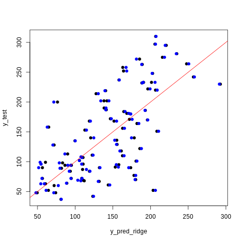
%%R

plot(y_pred_ridge, y_test, type="p", pch=19)
points(y_pred, y_test, col="blue", pch=19)
abline(a = 0, b = 1, col="red")
Citation
For attribution, please cite this work as:
T. Moudiki (2025-02-17). tisthemachinelearner: A Lightweight interface to scikit-learn with 2 classes, Classifier and Regressor (in Python and R). Retrieved from https://thierrymoudiki.github.io/blog/2025/02/17/python/r/tisthemllearner
BibTeX citation (remove empty spaces)
        @misc{ tmoudiki20250217,
          author = { T. Moudiki },
          title = { tisthemachinelearner: A Lightweight interface to scikit-learn with 2 classes, Classifier and Regressor (in Python and R) },
          url = { https://thierrymoudiki.github.io/blog/2025/02/17/python/r/tisthemllearner },
          year = { 2025 } }

Previous publications
- My last R posts: How conformalization helps weak models, fast conformal prediction with jackknife+ (and no refitting), and sklearn in R Jul 13, 2026
- Natively Interpretable Boosting Jul 12, 2026
- Fast conformal prediction (no refitting) for some Machine Learning models via closed-form jackknife plus Jun 27, 2026
- Using scikit-learn models in R easily with the tisthemachinelearner package Jun 21, 2026
- No-Code Machine Learning in Excel with the Techtonique API Jun 14, 2026
- How Conformal Prediction Makes Linear Models Good Enough — An Example Using R Package mlS3 Jun 7, 2026
- Techtonique dot net, the Machine Learning web API, is back online (but more like a passion project for now) May 31, 2026
- Conformalized TabICL: Prediction Intervals for a State-Of-The-Art Tabular Foundation Model in Python and R May 21, 2026
- Conformalized TabPFN: Prediction Intervals for a Pretrained Transformer for Tabular Data in Python and R May 17, 2026
- Probabilistic Time Series Cross-Validation with R package crossvalidation May 16, 2026
- One interface, (Almost) Every Classifier (and Regressor): unifiedml v0.3.0 May 9, 2026
- You Don't Need to Learn All the Weights on tabular data: The Case for rvflnet (a nonlinear expressive glmnet) on regression, classification and survival analysis May 2, 2026
- Survival analysis with sklearn, glmnet, keras, pytorch, lightgbm, xgboost, nnetsauce, mlsauce Part 2 Apr 28, 2026
- Any Sklearn Regressor as a Survival Model — Does It Actually Work? Benchmarking vs Established Packages Apr 26, 2026
- Conformal Optimization Beats Bayesian Optimization, Optuna and Random Search on 72 classification Datasets Apr 19, 2026
- `mlS3` — A Unified S3 Machine Learning Interface in R Apr 12, 2026
- One interface, (Almost) Every Classifier: unifiedml v0.2.1 Apr 4, 2026
- Techtonique dot net is down until further notice Apr 1, 2026
- Explaining Time-Series Forecasts with Sensitivity Analysis (ahead::dynrmf and external regressors) Mar 29, 2026
- Python version of 'Option pricing using time series models as market price of risk Pt.3' Mar 22, 2026
- Option pricing using time series models as market price of risk Pt.3 Mar 16, 2026
- Explaining Time-Series Forecasts with Exact Shapley Values (ahead::dynrmf with external regressors applied to scenarios) Mar 8, 2026
- My Presentation at Risk 2026: Lightweight Transfer Learning for Financial Forecasting Mar 1, 2026
- nnetsauce with and without jax for GPU acceleration Feb 23, 2026
- Understanding Boosted Configuration Networks (combined neural networks and boosting): An Intuitive Guide Through Their Hyperparameters Feb 16, 2026
- R version of Python package survivalist, for model-agnostic survival analysis Feb 9, 2026
- Presenting Lightweight Transfer Learning for Financial Forecasting (Risk 2026) Feb 4, 2026
- Option pricing using time series models as market price of risk Feb 1, 2026
- Enhancing Time Series Forecasting (ahead::ridge2f) with Attention-Based Context Vectors (ahead::contextridge2f) Jan 31, 2026
- Overfitting and scaling (on GPU T4) tests on nnetsauce.CustomRegressor Jan 29, 2026
- Beyond Cross-validation: Hyperparameter Optimization via Generalization Gap Modeling Jan 25, 2026
- GPopt for Machine Learning (hyperparameters' tuning) Jan 21, 2026
- rtopy: an R to Python bridge -- novelties Jan 8, 2026
- Python examples for 'Beyond Nelson-Siegel and splines: A model- agnostic Machine Learning framework for discount curve calibration, interpolation and extrapolation' Jan 3, 2026
- Forecasting benchmark: Dynrmf (a new serious competitor in town) vs Theta Method on M-Competitions and Tourism competitition Jan 1, 2026
- Finally figured out a way to port python packages to R using uv and reticulate: example with nnetsauce Dec 17, 2025
- Overfitting Random Fourier Features: Universal Approximation Property Dec 13, 2025
- Counterfactual Scenario Analysis with ahead::ridge2f Dec 11, 2025
- Zero-Shot Probabilistic Time Series Forecasting with TabPFN 2.5 and nnetsauce Dec 10, 2025
- ARIMA Pricing: Semi-Parametric Market price of risk for Risk-Neutral Pricing (code + preprint) Dec 7, 2025
- Analyzing Paper Reviews with LLMs: I Used ChatGPT, DeepSeek, Qwen, Mistral, Gemini, and Claude (and you should too + publish the analysis) Dec 3, 2025
- tisthemachinelearner: New Workflow with uv for R Integration of scikit-learn Dec 1, 2025
- (ICYMI) RPweave: Unified R + Python + LaTeX System using uv Nov 21, 2025
- unifiedml: A Unified Machine Learning Interface for R, is now on CRAN + Discussion about AI replacing humans Nov 16, 2025
- Context-aware Theta forecasting Method: Extending Classical Time Series Forecasting with Machine Learning Nov 13, 2025
- unifiedml in R: A Unified Machine Learning Interface Nov 5, 2025
- Deterministic Shift Adjustment in Arbitrage-Free Pricing (historical to risk-neutral short rates) Oct 28, 2025
- New instantaneous short rates models with their deterministic shift adjustment, for historical and risk-neutral simulation Oct 27, 2025
- RPweave: Unified R + Python + LaTeX System using uv Oct 19, 2025
- GAN-like Synthetic Data Generation Examples (on univariate, multivariate distributions, digits recognition, Fashion-MNIST, stock returns, and Olivetti faces) with DistroSimulator Oct 19, 2025
- R port of llama2.c Oct 9, 2025
- Native uncertainty quantification for time series with NGBoost Oct 8, 2025
- NGBoost (Natural Gradient Boosting) for Regression, Classification, Time Series forecasting and Reserving Oct 6, 2025
- Real-time pricing with a pretrained probabilistic stock return model Oct 1, 2025
- Combining any model with GARCH(1,1) for probabilistic stock forecasting Sep 23, 2025
- Generating Synthetic Data with R-vine Copulas using esgtoolkit in R Sep 21, 2025
- Reimagining Equity Solvency Capital Requirement Approximation (one of my Master's Thesis subjects): From Bilinear Interpolation to Probabilistic Machine Learning Sep 16, 2025
- Transfer Learning using ahead::ridge2f on synthetic stocks returns Pt.2: synthetic data generation Sep 9, 2025
- Transfer Learning using ahead::ridge2f on synthetic stocks returns Sep 8, 2025
- I'm supposed to present 'Conformal Predictive Simulations for Univariate Time Series' at COPA CONFERENCE 2025 in London... Sep 4, 2025
- external regressors in ahead::dynrmf's interface for Machine learning forecasting Sep 1, 2025
- Another interesting decision, now for 'Beyond Nelson-Siegel and splines: A model-agnostic Machine Learning framework for discount curve calibration, interpolation and extrapolation' Aug 20, 2025
- Boosting any randomized based learner for regression, classification and univariate/multivariate time series forcasting Jul 26, 2025
- New nnetsauce version with CustomBackPropRegressor (CustomRegressor with Backpropagation) and ElasticNet2Regressor (Ridge2 with ElasticNet regularization) Jul 15, 2025
- mlsauce (home to a model-agnostic gradient boosting algorithm) can now be installed from PyPI. Jul 10, 2025
- A user-friendly graphical interface to techtonique dot net's API (will eventually contain graphics). Jul 8, 2025
- Calling =TECHTO_MLCLASSIFICATION for Machine Learning supervised CLASSIFICATION in Excel is just a matter of copying and pasting Jul 7, 2025
- Calling =TECHTO_MLREGRESSION for Machine Learning supervised regression in Excel is just a matter of copying and pasting Jul 6, 2025
- Calling =TECHTO_RESERVING and =TECHTO_MLRESERVING for claims triangle reserving in Excel is just a matter of copying and pasting Jul 5, 2025
- Calling =TECHTO_SURVIVAL for Survival Analysis in Excel is just a matter of copying and pasting Jul 4, 2025
- Calling =TECHTO_SIMULATION for Stochastic Simulation in Excel is just a matter of copying and pasting Jul 3, 2025
- Calling =TECHTO_FORECAST for forecasting in Excel is just a matter of copying and pasting Jul 2, 2025
- Random Vector Functional Link (RVFL) artificial neural network with 2 regularization parameters successfully used for forecasting/synthetic simulation in professional settings: Extensions (including Bayesian) Jul 1, 2025
- R version of 'Backpropagating quasi-randomized neural networks' Jun 24, 2025
- Backpropagating quasi-randomized neural networks Jun 23, 2025
- Beyond ARMA-GARCH: leveraging any statistical model for volatility forecasting Jun 21, 2025
- Stacked generalization (Machine Learning model stacking) + conformal prediction for forecasting with ahead::mlf Jun 18, 2025
- An Overfitting dilemma: XGBoost Default Hyperparameters vs GenericBooster + LinearRegression Default Hyperparameters Jun 14, 2025
- Programming language-agnostic reserving using RidgeCV, LightGBM, XGBoost, and ExtraTrees Machine Learning models Jun 13, 2025
- Free R, Python and SQL editors in techtonique dot net Jun 9, 2025
- Beyond Nelson-Siegel and splines: A model-agnostic Machine Learning framework for discount curve calibration, interpolation and extrapolation Jun 7, 2025
- scikit-learn, glmnet, xgboost, lightgbm, pytorch, keras, nnetsauce in probabilistic Machine Learning (for longitudinal data) Reserving (work in progress) Jun 6, 2025
- R version of Probabilistic Machine Learning (for longitudinal data) Reserving (work in progress) Jun 5, 2025
- Probabilistic Machine Learning (for longitudinal data) Reserving (work in progress) Jun 4, 2025
- Python version of Beyond ARMA-GARCH: leveraging model-agnostic Quasi-Randomized networks and conformal prediction for nonparametric probabilistic stock forecasting (ML-ARCH) Jun 3, 2025
- Beyond ARMA-GARCH: leveraging model-agnostic Machine Learning and conformal prediction for nonparametric probabilistic stock forecasting (ML-ARCH) Jun 2, 2025
- Permutations and SHAPley values for feature importance in techtonique dot net's API (with R + Python + the command line) Jun 1, 2025
- Which patient is going to survive longer? Another guide to using techtonique dot net's API (with R + Python + the command line) for survival analysis May 31, 2025
- A Guide to Using techtonique.net's API and rush for simulating and plotting Stochastic Scenarios May 30, 2025
- Simulating Stochastic Scenarios with Diffusion Models: A Guide to Using techtonique.net's API for the purpose May 29, 2025
- Will my apartment in 5th avenue be overpriced or not? Harnessing the power of www.techtonique.net (+ xgboost, lightgbm, catboost) to find out May 28, 2025
- How long must I wait until something happens: A Comprehensive Guide to Survival Analysis via an API May 27, 2025
- Harnessing the Power of techtonique.net: A Comprehensive Guide to Machine Learning Classification via an API May 26, 2025
- Quantile regression with any regressor -- Examples with RandomForestRegressor, RidgeCV, KNeighborsRegressor May 20, 2025
- Survival stacking: survival analysis translated as supervised classification in R and Python May 5, 2025
- 'Bayesian' optimization of hyperparameters in a R machine learning model using the bayesianrvfl package Apr 25, 2025
- A lightweight interface to scikit-learn in R: Bayesian and Conformal prediction Apr 21, 2025
- A lightweight interface to scikit-learn in R Pt.2: probabilistic time series forecasting in conjunction with ahead::dynrmf Apr 20, 2025
- Extending the Theta forecasting method to GLMs, GAMs, GLMBOOST and attention: benchmarking on Tourism, M1, M3 and M4 competition data sets (28000 series) Apr 14, 2025
- Extending the Theta forecasting method to GLMs and attention Apr 8, 2025
- Nonlinear conformalized Generalized Linear Models (GLMs) with R package 'rvfl' (and other models) Mar 31, 2025
- Probabilistic Time Series Forecasting (predictive simulations) in Microsoft Excel using Python, xlwings lite and www.techtonique.net Mar 28, 2025
- Conformalize (improved prediction intervals and simulations) any R Machine Learning model with misc::conformalize Mar 25, 2025
- My poster for the 18th FINANCIAL RISKS INTERNATIONAL FORUM by Institut Louis Bachelier/Fondation du Risque/Europlace Institute of Finance Mar 19, 2025
- Interpretable probabilistic kernel ridge regression using Matérn 3/2 kernels Mar 16, 2025
- (News from) Probabilistic Forecasting of univariate and multivariate Time Series using Quasi-Randomized Neural Networks (Ridge2) and Conformal Prediction Mar 9, 2025
- Word-Online: re-creating Karpathy's char-RNN (with supervised linear online learning of word embeddings) for text completion Mar 8, 2025
- CRAN-like repository for most recent releases of Techtonique's R packages Mar 2, 2025
- Presenting 'Online Probabilistic Estimation of Carbon Beta and Carbon Shapley Values for Financial and Climate Risk' at Institut Louis Bachelier Feb 27, 2025
- Web app with DeepSeek R1 and Hugging Face API for chatting Feb 23, 2025
- tisthemachinelearner: A Lightweight interface to scikit-learn with 2 classes, Classifier and Regressor (in Python and R) Feb 17, 2025
- R version of survivalist: Probabilistic model-agnostic survival analysis using scikit-learn, xgboost, lightgbm (and conformal prediction) Feb 12, 2025
- Model-agnostic global Survival Prediction of Patients with Myeloid Leukemia in QRT/Gustave Roussy Challenge (challengedata.ens.fr): Python's survivalist Quickstart Feb 10, 2025
- A simple test of the martingale hypothesis in esgtoolkit Feb 3, 2025
- Command Line Interface (CLI) for techtonique.net's API Jan 31, 2025
- Gradient-Boosting and Boostrap aggregating anything (alert: high performance): Part5, easier install and Rust backend Jan 27, 2025
- Just got a paper on conformal prediction REJECTED by International Journal of Forecasting despite evidence on 30,000 time series (and more). What's going on? Part2: 1311 time series from the Tourism competition Jan 20, 2025
- Techtonique is released! (with a tutorial in various programming languages and formats) Jan 14, 2025
- Univariate and Multivariate Probabilistic Forecasting with nnetsauce and TabPFN Jan 14, 2025
- Just got a paper on conformal prediction REJECTED by International Journal of Forecasting despite evidence on 30,000 time series (and more). What's going on? Jan 5, 2025
- Python and Interactive dashboard version of Stock price forecasting with Deep Learning: throwing power at the problem (and why it won't make you rich) Dec 31, 2024
- Stock price forecasting with Deep Learning: throwing power at the problem (and why it won't make you rich) Dec 29, 2024
- No-code Machine Learning Cross-validation and Interpretability in techtonique.net Dec 23, 2024
- survivalist: Probabilistic model-agnostic survival analysis using scikit-learn, glmnet, xgboost, lightgbm, pytorch, keras, nnetsauce and mlsauce Dec 15, 2024
- Model-agnostic 'Bayesian' optimization (for hyperparameter tuning) using conformalized surrogates in GPopt Dec 9, 2024
- You can beat Forecasting LLMs (Large Language Models a.k.a foundation models) with nnetsauce.MTS Pt.2: Generic Gradient Boosting Dec 1, 2024
- You can beat Forecasting LLMs (Large Language Models a.k.a foundation models) with nnetsauce.MTS Nov 24, 2024
- Unified interface and conformal prediction (calibrated prediction intervals) for R package forecast (and 'affiliates') Nov 23, 2024
- GLMNet in Python: Generalized Linear Models Nov 18, 2024
- Gradient-Boosting anything (alert: high performance): Part4, Time series forecasting Nov 10, 2024
- Predictive scenarios simulation in R, Python and Excel using Techtonique API Nov 3, 2024
- Chat with your tabular data in www.techtonique.net Oct 30, 2024
- Gradient-Boosting anything (alert: high performance): Part3, Histogram-based boosting Oct 28, 2024
- R editor and SQL console (in addition to Python editors) in www.techtonique.net Oct 21, 2024
- R and Python consoles + JupyterLite in www.techtonique.net Oct 15, 2024
- Gradient-Boosting anything (alert: high performance): Part2, R version Oct 14, 2024
- Gradient-Boosting anything (alert: high performance) Oct 6, 2024
- Benchmarking 30 statistical/Machine Learning models on the VN1 Forecasting -- Accuracy challenge Oct 4, 2024
- Automated random variable distribution inference using Kullback-Leibler divergence and simulating best-fitting distribution Oct 2, 2024
- Forecasting in Excel using Techtonique's Machine Learning APIs under the hood Sep 30, 2024
- Techtonique web app for data-driven decisions using Mathematics, Statistics, Machine Learning, and Data Visualization Sep 25, 2024
- Parallel for loops (Map or Reduce) + New versions of nnetsauce and ahead Sep 16, 2024
- Adaptive (online/streaming) learning with uncertainty quantification using Polyak averaging in learningmachine Sep 10, 2024
- New versions of nnetsauce and ahead Sep 9, 2024
- Prediction sets and prediction intervals for conformalized Auto XGBoost, Auto LightGBM, Auto CatBoost, Auto GradientBoosting Sep 2, 2024
- Quick/automated R package development workflow (assuming you're using macOS or Linux) Part2 Aug 30, 2024
- R package development workflow (assuming you're using macOS or Linux) Aug 27, 2024
- A new method for deriving a nonparametric confidence interval for the mean Aug 26, 2024
- Conformalized adaptive (online/streaming) learning using learningmachine in Python and R Aug 19, 2024
- Bayesian (nonlinear) adaptive learning Aug 12, 2024
- Auto XGBoost, Auto LightGBM, Auto CatBoost, Auto GradientBoosting Aug 5, 2024
- Copulas for uncertainty quantification in time series forecasting Jul 28, 2024
- Forecasting uncertainty: sequential split conformal prediction + Block bootstrap (web app) Jul 22, 2024
- learningmachine for Python (new version) Jul 15, 2024
- learningmachine v2.0.0: Machine Learning with explanations and uncertainty quantification Jul 8, 2024
- My presentation at ISF 2024 conference (slides with nnetsauce probabilistic forecasting news) Jul 3, 2024
- 10 uncertainty quantification methods in nnetsauce forecasting Jul 1, 2024
- Forecasting with XGBoost embedded in Quasi-Randomized Neural Networks Jun 24, 2024
- Forecasting Monthly Airline Passenger Numbers with Quasi-Randomized Neural Networks Jun 17, 2024
- Automated hyperparameter tuning using any conformalized surrogate Jun 9, 2024
- Recognizing handwritten digits with Ridge2Classifier Jun 3, 2024
- Forecasting the Economy May 27, 2024
- A detailed introduction to Deep Quasi-Randomized 'neural' networks May 19, 2024
- Probability of receiving a loan; using learningmachine May 12, 2024
- mlsauce's `v0.18.2`: various examples and benchmarks with dimension reduction May 6, 2024
- mlsauce's `v0.17.0`: boosting with Elastic Net, polynomials and heterogeneity in explanatory variables Apr 29, 2024
- mlsauce's `v0.13.0`: taking into account inputs heterogeneity through clustering Apr 21, 2024
- mlsauce's `v0.12.0`: prediction intervals for LSBoostRegressor Apr 15, 2024
- Conformalized predictive simulations for univariate time series on more than 250 data sets Apr 7, 2024
- learningmachine v1.1.2: for Python Apr 1, 2024
- learningmachine v1.0.0: prediction intervals around the probability of the event 'a tumor being malignant' Mar 25, 2024
- Bayesian inference and conformal prediction (prediction intervals) in nnetsauce v0.18.1 Mar 18, 2024
- Multiple examples of Machine Learning forecasting with ahead Mar 11, 2024
- rtopy (v0.1.1): calling R functions in Python Mar 4, 2024
- ahead forecasting (v0.10.0): fast time series model calibration and Python plots Feb 26, 2024
- A plethora of datasets at your fingertips Part3: how many times do couples cheat on each other? Feb 19, 2024
- nnetsauce's introduction as of 2024-02-11 (new version 0.17.0) Feb 11, 2024
- Tuning Machine Learning models with GPopt's new version Part 2 Feb 5, 2024
- Tuning Machine Learning models with GPopt's new version Jan 29, 2024
- Subsampling continuous and discrete response variables Jan 22, 2024
- DeepMTS, a Deep Learning Model for Multivariate Time Series Jan 15, 2024
- A classifier that's very accurate (and deep) Pt.2: there are > 90 classifiers in nnetsauce Jan 8, 2024
- learningmachine: prediction intervals for conformalized Kernel ridge regression and Random Forest Jan 1, 2024
- A plethora of datasets at your fingertips Part2: how many times do couples cheat on each other? Descriptive analytics, interpretability and prediction intervals using conformal prediction Dec 25, 2023
- Diffusion models in Python with esgtoolkit (Part2) Dec 18, 2023
- Diffusion models in Python with esgtoolkit Dec 11, 2023
- Julia packaging at the command line Dec 4, 2023
- Quasi-randomized nnetworks in Julia, Python and R Nov 27, 2023
- A plethora of datasets at your fingertips Nov 20, 2023
- A classifier that's very accurate (and deep) Nov 12, 2023
- mlsauce version 0.8.10: Statistical/Machine Learning with Python and R Nov 5, 2023
- AutoML in nnetsauce (randomized and quasi-randomized nnetworks) Pt.2: multivariate time series forecasting Oct 29, 2023
- AutoML in nnetsauce (randomized and quasi-randomized nnetworks) Oct 22, 2023
- Version v0.14.0 of nnetsauce for R and Python Oct 16, 2023
- A diffusion model: G2++ Oct 9, 2023
- Diffusion models in ESGtoolkit + announcements Oct 2, 2023
- An infinity of time series forecasting models in nnetsauce (Part 2 with uncertainty quantification) Sep 25, 2023
- (News from) forecasting in Python with ahead (progress bars and plots) Sep 18, 2023
- Forecasting in Python with ahead Sep 11, 2023
- Risk-neutralize simulations Sep 4, 2023
- Comparing cross-validation results using crossval_ml and boxplots Aug 27, 2023
- Reminder Apr 30, 2023
- Did you ask ChatGPT about who you are? Apr 16, 2023
- A new version of nnetsauce (randomized and quasi-randomized 'neural' networks) Apr 2, 2023
- Simple interfaces to the forecasting API Nov 23, 2022
- A web application for forecasting in Python, R, Ruby, C#, JavaScript, PHP, Go, Rust, Java, MATLAB, etc. Nov 2, 2022
- Prediction intervals (not only) for Boosted Configuration Networks in Python Oct 5, 2022
- Boosted Configuration (neural) Networks Pt. 2 Sep 3, 2022
- Boosted Configuration (_neural_) Networks for classification Jul 21, 2022
- A Machine Learning workflow using Techtonique Jun 6, 2022
- Super Mario Bros © in the browser using PyScript May 8, 2022
- News from ESGtoolkit, ycinterextra, and nnetsauce Apr 4, 2022
- Explaining a Keras _neural_ network predictions with the-teller Mar 11, 2022
- New version of nnetsauce -- various quasi-randomized networks Feb 12, 2022
- A dashboard illustrating bivariate time series forecasting with `ahead` Jan 14, 2022
- Hundreds of Statistical/Machine Learning models for univariate time series, using ahead, ranger, xgboost, and caret Dec 20, 2021
- Forecasting with `ahead` (Python version) Dec 13, 2021
- Tuning and interpreting LSBoost Nov 15, 2021
- Time series cross-validation using `crossvalidation` (Part 2) Nov 7, 2021
- Fast and scalable forecasting with ahead::ridge2f Oct 31, 2021
- Automatic Forecasting with `ahead::dynrmf` and Ridge regression Oct 22, 2021
- Forecasting with `ahead` Oct 15, 2021
- Classification using linear regression Sep 26, 2021
- `crossvalidation` and random search for calibrating support vector machines Aug 6, 2021
- parallel grid search cross-validation using `crossvalidation` Jul 31, 2021
- `crossvalidation` on R-universe, plus a classification example Jul 23, 2021
- Documentation and source code for GPopt, a package for Bayesian optimization Jul 2, 2021
- Hyperparameters tuning with GPopt Jun 11, 2021
- A forecasting tool (API) with examples in curl, R, Python May 28, 2021
- Bayesian Optimization with GPopt Part 2 (save and resume) Apr 30, 2021
- Bayesian Optimization with GPopt Apr 16, 2021
- Compatibility of nnetsauce and mlsauce with scikit-learn Mar 26, 2021
- Explaining xgboost predictions with the teller Mar 12, 2021
- An infinity of time series models in nnetsauce Mar 6, 2021
- New activation functions in mlsauce's LSBoost Feb 12, 2021
- 2020 recap, Gradient Boosting, Generalized Linear Models, AdaOpt with nnetsauce and mlsauce Dec 29, 2020
- A deeper learning architecture in nnetsauce Dec 18, 2020
- Classify penguins with nnetsauce's MultitaskClassifier Dec 11, 2020
- Bayesian forecasting for uni/multivariate time series Dec 4, 2020
- Generalized nonlinear models in nnetsauce Nov 28, 2020
- Boosting nonlinear penalized least squares Nov 21, 2020
- Statistical/Machine Learning explainability using Kernel Ridge Regression surrogates Nov 6, 2020
- NEWS Oct 30, 2020
- A glimpse into my PhD journey Oct 23, 2020
- Submitting R package to CRAN Oct 16, 2020
- Simulation of dependent variables in ESGtoolkit Oct 9, 2020
- Forecasting lung disease progression Oct 2, 2020
- New nnetsauce Sep 25, 2020
- Technical documentation Sep 18, 2020
- A new version of nnetsauce, and a new Techtonique website Sep 11, 2020
- Back next week, and a few announcements Sep 4, 2020
- Explainable 'AI' using Gradient Boosted randomized networks Pt2 (the Lasso) Jul 31, 2020
- LSBoost: Explainable 'AI' using Gradient Boosted randomized networks (with examples in R and Python) Jul 24, 2020
- nnetsauce version 0.5.0, randomized neural networks on GPU Jul 17, 2020
- Maximizing your tip as a waiter (Part 2) Jul 10, 2020
- New version of mlsauce, with Gradient Boosted randomized networks and stump decision trees Jul 3, 2020
- Announcements Jun 26, 2020
- Parallel AdaOpt classification Jun 19, 2020
- Comments section and other news Jun 12, 2020
- Maximizing your tip as a waiter Jun 5, 2020
- AdaOpt classification on MNIST handwritten digits (without preprocessing) May 29, 2020
- AdaOpt (a probabilistic classifier based on a mix of multivariable optimization and nearest neighbors) for R May 22, 2020
- AdaOpt May 15, 2020
- Custom errors for cross-validation using crossval::crossval_ml May 8, 2020
- Documentation+Pypi for the `teller`, a model-agnostic tool for Machine Learning explainability May 1, 2020
- Encoding your categorical variables based on the response variable and correlations Apr 24, 2020
- Linear model, xgboost and randomForest cross-validation using crossval::crossval_ml Apr 17, 2020
- Grid search cross-validation using crossval Apr 10, 2020
- Documentation for the querier, a query language for Data Frames Apr 3, 2020
- Time series cross-validation using crossval Mar 27, 2020
- On model specification, identification, degrees of freedom and regularization Mar 20, 2020
- Import data into the querier (now on Pypi), a query language for Data Frames Mar 13, 2020
- R notebooks for nnetsauce Mar 6, 2020
- Version 0.4.0 of nnetsauce, with fruits and breast cancer classification Feb 28, 2020
- Create a specific feed in your Jekyll blog Feb 21, 2020
- Git/Github for contributing to package development Feb 14, 2020
- Feedback forms for contributing Feb 7, 2020
- nnetsauce for R Jan 31, 2020
- A new version of nnetsauce (v0.3.1) Jan 24, 2020
- ESGtoolkit, a tool for Monte Carlo simulation (v0.2.0) Jan 17, 2020
- Search bar, new year 2020 Jan 10, 2020
- 2019 Recap, the nnetsauce, the teller and the querier Dec 20, 2019
- Understanding model interactions with the `teller` Dec 13, 2019
- Using the `teller` on a classifier Dec 6, 2019
- Benchmarking the querier's verbs Nov 29, 2019
- Composing the querier's verbs for data wrangling Nov 22, 2019
- Comparing and explaining model predictions with the teller Nov 15, 2019
- Tests for the significance of marginal effects in the teller Nov 8, 2019
- Introducing the teller Nov 1, 2019
- Introducing the querier Oct 25, 2019
- Prediction intervals for nnetsauce models Oct 18, 2019
- Using R in Python for statistical learning/data science Oct 11, 2019
- Model calibration with `crossval` Oct 4, 2019
- Bagging in the nnetsauce Sep 25, 2019
- Adaboost learning with nnetsauce Sep 18, 2019
- Change in blog's presentation Sep 4, 2019
- nnetsauce on Pypi Jun 5, 2019
- More nnetsauce (examples of use) May 9, 2019
- nnetsauce Mar 13, 2019
- crossval Mar 13, 2019
- test Mar 10, 2019
Comments powered by Talkyard.