As mentioned here 2 weeks ago, when introducting the teller, there is an increasing need for transparency and fairness in Statistical/Machine Learning (ML) models predictions. Some ML models which are not linear are considered as being black boxes, but they may exhibit high accuracy numbers. Since we do not want to sacrifice this high accuracy to explainability, we can use the teller, a model-agnostic tool for ML explainability, to understand them a little bit more.
In this post, we are going to use the teller to compare two ML models on the Boston Housing dataset:
- Extremely Randomized Trees
- Random Forest Regressions
Why am I using this dataset this much? Not because I’m a real estate agent, but:
- It’s widely used and well-studied in ML
- It’s directly available to everyone through (the also widely used) R package
MASS, and Python’s scikit-learn - It has a moderate size, ideal for demos
- It allows to derive insights which are interesting, and understandable by almost everyone
I also found the paper: Harrison, D. and Rubinfeld, D.L. (1978) Hedonic prices and the demand for clean air. J. Environ. Economics and Management 5, 81–102, to be an interesting and accessible read. If you are interested.
Data description: The response (variable to be explained) is MEDV, Median value of owner-occupied homes in $1000’s.
- CRIM per capita crime rate by town
- ZN proportion of residential land zoned for lots over 25,000 sq.ft.
- INDUS proportion of non-retail business acres per town
- CHAS Charles River dummy variable (= 1 if tract bounds river; 0 otherwise)
- NOX nitric oxides concentration (parts per 10 million)
- RM average number of rooms per dwelling
- AGE proportion of owner-occupied units built prior to 1940
- DIS weighted distances to five Boston employment centres
- RAD index of accessibility to radial highways
- TAX full-value property-tax rate per $10,000
- PTRATIO pupil-teacher ratio by town
- LSTAT % lower status of the population
- MEDV Median value of owner-occupied homes in $1000’s (the reponse)
Install the package and import data
Currently, the teller’s development version can be obtained from Github as:
!pip install git+https://github.com/Techtonique/teller.git
Packages and dataset:
# Import packages and data
import teller as tr
import pandas as pd
import numpy as np
import lightgbm as lgb
import xgboost as xgb
import math

from sklearn import datasets, linear_model
from sklearn.ensemble import RandomForestRegressor, ExtraTreesRegressor, BaggingRegressor
from sklearn import datasets
from sklearn.model_selection import train_test_split, GridSearchCV
from sklearn import metrics

# import data
boston = datasets.load_boston()
X = np.delete(boston.data, 11, 1)
y = boston.target
col_names = np.append(np.delete(boston.feature_names, 11), 'MEDV')
Model training and explanations
We split data into a training and a testing set:
X_train, X_test, y_train, y_test = train_test_split(X, y, test_size=0.2,
                                                    random_state=123)
print(X_train.shape)
print(X_test.shape)
print("mean of y_test: ")
print(np.mean(y_test))
print("std. deviation of y_test: ")
print(np.std(y_test))
Now we train our 2 models, starting with the Extremely Randomized Trees:
# fit an Extra Trees model to Boston Housing data
regr2 = ExtraTreesRegressor(n_estimators=1000,
                            max_features=int(math.sqrt(X_train.shape[1])),
                            random_state=123)
regr2.fit(X_train, y_train)


# creating the explainer
expr2 = tr.Explainer(obj=regr2)


# fitting the explainer (for heterogeneity of effects only)
expr2.fit(X_test, y_test, X_names=col_names[:-1], y_name=col_names[-1], method="avg")


# confidence intervals and tests on marginal effects (Jackknife)
expr2.fit(X_test, y_test, X_names=col_names[:-1], y_name=col_names[-1], method="ci")


# summary of results for the model
print(expr2.summary())
Score (rmse):
 10.813


Residuals:
     Min       1Q    Median        3Q       Max
-11.7904 -1.84795 -0.288655  0.937975  18.51445


Tests on marginal effects (Jackknife):
          Estimate   Std. Error   95% lbound   95% ubound     Pr(>|t|)
NOX       -59.4205  2.22045e-16     -59.4205     -59.4205            0  ***
PTRATIO   -2.00072     0.390455     -2.77528     -1.22616  1.44031e-06  ***
CRIM             0  2.22045e-16 -4.40477e-16  4.40477e-16            1    -
ZN               0  2.22045e-16 -4.40477e-16  4.40477e-16            1    -
CHAS             0  2.22045e-16 -4.40477e-16  4.40477e-16            1    -
RAD              0  2.22045e-16 -4.40477e-16  4.40477e-16            1    -
TAX      0.0121302  2.22045e-16    0.0121302    0.0121302            0  ***
INDUS    0.0125259  3.31241e-16    0.0125259    0.0125259            0  ***
LSTAT     0.127336      0.27273    -0.413686     0.668359      0.64158    -
AGE       0.643206  6.69456e-15     0.643206     0.643206            0  ***
DIS        1.17726  2.45467e-14      1.17726      1.17726            0  ***
RM         7.29791     0.201907      6.89738      7.69844  1.37027e-59  ***


Signif. codes:  0 ‘***’ 0.001 ‘**’ 0.01 ‘*’ 0.05 ‘.’ 0.1 ‘-’ 1


Multiple R-squared:  0.869,	Adjusted R-squared:  0.852


Heterogeneity of marginal effects:
              mean         std          min         max
NOX     -58.837937  476.247650 -4564.951708  755.791176
PTRATIO  -1.818289   19.700286  -130.395492   38.014987
CRIM      0.000000    0.000000     0.000000    0.000000
ZN        0.000000    0.000000     0.000000    0.000000
CHAS      0.000000    0.000000     0.000000    0.000000
RAD       0.000000    0.000000     0.000000    0.000000
TAX       0.012011    0.102841     0.000000    1.020264
INDUS     0.012403    0.125266     0.000000    1.265120
LSTAT     0.128762    2.955437    -8.391279   27.818439
AGE       0.636900    4.638587    -1.521252   34.266627
DIS       1.165723   14.435157   -24.558015  143.461713
RM        7.228340   28.794942     0.000000  215.621069
None
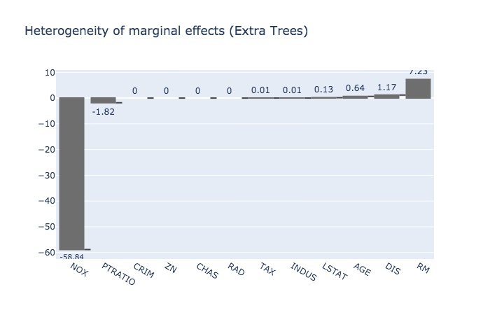
Extra Trees predictions for home value are highly sensisitive to air pollution. And increase of 1 in nitrogen oxides concentration (parts per 10 million) leads, all else held constant and on average, to a decrease of 58k$ in median homes’ values. The increase in home value is driven by the number of rooms. We can also note that variables such as criminality rate and the accessibility to radial highways, seem to have a negligible impact on model predictions.
Now, we’ll train a Random Forest on the same dataset, and see what it tells us about its predictions:
# fit a random forest model
regr1 = RandomForestRegressor(n_estimators=1000,
                              max_features=int(math.sqrt(X_train.shape[1])),
                              random_state=123)
regr1.fit(X_train, y_train)


# creating the explainer
expr1 = tr.Explainer(obj=regr1)


# fitting the explainer (for heterogeneity of effects only)
expr1.fit(X_test, y_test, X_names=col_names[:-1], y_name=col_names[-1], method="avg")


# confidence intervals and tests on marginal effects (Jackknife)
expr1.fit(X_test, y_test, X_names=col_names[:-1], y_name=col_names[-1], method="ci")


# summary of results for the model
print(expr1.summary())
Score (rmse):
 13.639


Residuals:
     Min     1Q  Median       3Q      Max
-10.6667 -1.396 -0.5047  1.25705  22.4512


Tests on marginal effects (Jackknife):
         Estimate   Std. Error   95% lbound   95% ubound     Pr(>|t|)
NOX      -65.9852      23.5248     -112.652     -19.3183   0.00603773   **
PTRATIO  -19.0443      5.74131     -30.4335      -7.6551   0.00126512   **
LSTAT      -2.972      3.11832     -9.15791      3.21392     0.342827    -
INDUS    -1.90767      2.88467     -7.63009      3.81474     0.509917    -
ZN      -0.670289     0.429838     -1.52297     0.182394      0.12203    -
TAX     -0.412312    0.0252358    -0.462373    -0.362251  4.10351e-30  ***
CHAS            0  2.22045e-16 -4.40477e-16  4.40477e-16            1    -
AGE      0.583416   5.5788e-15     0.583416     0.583416            0  ***
CRIM      4.74938  1.16039e-13      4.74938      4.74938            0  ***
DIS       10.7329  2.14226e-13      10.7329      10.7329            0  ***
RAD       20.1803      4.93784       10.385      29.9757  8.78367e-05  ***
RM        31.1946     0.809636      29.5885      32.8007  3.33135e-62  ***


Signif. codes:  0 ‘***’ 0.001 ‘**’ 0.01 ‘*’ 0.05 ‘.’ 0.1 ‘-’ 1


Multiple R-squared:  0.835,	Adjusted R-squared:  0.813


Heterogeneity of marginal effects:
              mean         std          min          max
NOX     -65.077408  837.110491 -7304.767586  2092.276204
PTRATIO -18.914731   81.475430  -585.195412    40.313679
LSTAT    -3.504697   51.609150  -260.521317   226.189605
INDUS    -1.917253   76.799856  -342.638186   617.598139
ZN       -0.667706    9.494545   -49.129261    41.635391
TAX      -0.408517    3.248658   -32.287535     0.880749
CHAS      0.000000    0.000000     0.000000     0.000000
AGE       0.577696   12.232191   -71.283614    85.560655
CRIM      4.702817   47.496127     0.000000   479.687370
DIS      10.627708   62.112145     0.000000   540.229275
RAD      20.011127  144.732678  -332.344998   623.404904
RM       30.895241  169.441083  -247.545527  1346.559346
None
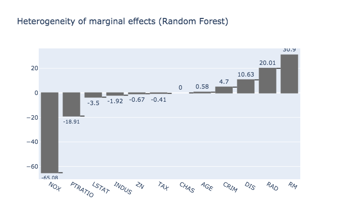
For this model too, air pollution is an important variable driving the decrease in home value. The lack of teachers for each kid plays a more important role here, but contrary to Extra Trees, Random Forests give much more importance to the accessibility of radial highways.
Comparing models
We can finally compare both models side by side, using the teller’s Comparator:
# create object for model comparison
# expr1 is for Random Forest
# expr2 is for Extra Trees
cpr = tr.Comparator(expr1, expr2)


# print summary of results for model comparison
print(cpr.summary())
Scores (rmse):
Object1: 13.639
Object2: 10.813


R-squared:
Object1:
Multiple:  0.835, Adjusted:  0.813
Object2:
Multiple:  0.869, Adjusted:  0.852


Residuals:
Object1:
     Min     1Q  Median       3Q      Max
-10.6667 -1.396 -0.5047  1.25705  22.4512
Object2:
     Min       1Q    Median        3Q       Max
-11.7904 -1.84795 -0.288655  0.937975  18.51445


Paired t-test (H0: mean(resids1) > mean(resids2) at 5%):
statistic: 0.18249
p.value: 0.57231
conf. int: [-inf, 0.90189]
mean of x: -0.11477
mean of y: -0.20446
alternative: less


Marginal effects:
        Estimate1  Std. Error1 Signif.  Estimate2  Std. Error2 Signif.
AGE      0.583416   5.5788e-15     ***   0.643206  6.69456e-15     ***
CHAS            0  2.22045e-16       -          0  2.22045e-16       -
CRIM      4.74938  1.16039e-13     ***          0  2.22045e-16       -
DIS       10.7329  2.14226e-13     ***    1.17726  2.45467e-14     ***
INDUS    -1.90767      2.88467       -  0.0125259  3.31241e-16     ***
LSTAT      -2.972      3.11832       -   0.127336      0.27273       -
NOX      -65.9852      23.5248      **   -59.4205  2.22045e-16     ***
PTRATIO  -19.0443      5.74131      **   -2.00072     0.390455     ***
RAD       20.1803      4.93784     ***          0  2.22045e-16       -
RM        31.1946     0.809636     ***    7.29791     0.201907     ***
TAX     -0.412312    0.0252358     ***  0.0121302  2.22045e-16     ***
ZN      -0.670289     0.429838       -          0  2.22045e-16       -


Signif. codes:  0 ‘***’ 0.001 ‘**’ 0.01 ‘*’ 0.05 ‘.’ 0.1 ‘-’ 1
None
The first output is test set Root Mean Squared Error (RMSE) for both models, then we have information such as Multiple R-Squared and the distribution of residuals. Confidence interval (given by a Student t-test) around the difference of residuals means contains 0, so the null hypothesis is not rejected at 5%.
A notebook containing these results can be found here. Contributions/remarks are welcome as usual, you can submit a pull request on Github.
Note: I am currently looking for a gig. You can hire me on Malt or send me an email: thierry dot moudiki at pm dot me. I can do descriptive statistics, data preparation, feature engineering, model calibration, training and validation, and model outputs’ interpretation. I am fluent in Python, R, SQL, Microsoft Excel, Visual Basic (among others) and French. My résumé? Here!
For attribution, please cite this work as:
T. Moudiki (2019-11-15). Comparing and explaining model predictions with the teller. Retrieved from https://thierrymoudiki.github.io/blog/2019/11/15/explainableml/the-teller-3
BibTeX citation (remove empty spaces)
        @misc{ tmoudiki20191115,
          author = { T. Moudiki },
          title = { Comparing and explaining model predictions with the teller },
          url = { https://thierrymoudiki.github.io/blog/2019/11/15/explainableml/the-teller-3 },
          year = { 2019 } }

Previous publications
- My last R posts: How conformalization helps weak models, fast conformal prediction with jackknife+ (and no refitting), and sklearn in R Jul 13, 2026
- Natively Interpretable Boosting Jul 12, 2026
- Fast conformal prediction (no refitting) for some Machine Learning models via closed-form jackknife plus Jun 27, 2026
- Using scikit-learn models in R easily with the tisthemachinelearner package Jun 21, 2026
- No-Code Machine Learning in Excel with the Techtonique API Jun 14, 2026
- How Conformal Prediction Makes Linear Models Good Enough — An Example Using R Package mlS3 Jun 7, 2026
- Techtonique dot net, the Machine Learning web API, is back online (but more like a passion project for now) May 31, 2026
- Conformalized TabICL: Prediction Intervals for a State-Of-The-Art Tabular Foundation Model in Python and R May 21, 2026
- Conformalized TabPFN: Prediction Intervals for a Pretrained Transformer for Tabular Data in Python and R May 17, 2026
- Probabilistic Time Series Cross-Validation with R package crossvalidation May 16, 2026
- One interface, (Almost) Every Classifier (and Regressor): unifiedml v0.3.0 May 9, 2026
- You Don't Need to Learn All the Weights on tabular data: The Case for rvflnet (a nonlinear expressive glmnet) on regression, classification and survival analysis May 2, 2026
- Survival analysis with sklearn, glmnet, keras, pytorch, lightgbm, xgboost, nnetsauce, mlsauce Part 2 Apr 28, 2026
- Any Sklearn Regressor as a Survival Model — Does It Actually Work? Benchmarking vs Established Packages Apr 26, 2026
- Conformal Optimization Beats Bayesian Optimization, Optuna and Random Search on 72 classification Datasets Apr 19, 2026
- `mlS3` — A Unified S3 Machine Learning Interface in R Apr 12, 2026
- One interface, (Almost) Every Classifier: unifiedml v0.2.1 Apr 4, 2026
- Techtonique dot net is down until further notice Apr 1, 2026
- Explaining Time-Series Forecasts with Sensitivity Analysis (ahead::dynrmf and external regressors) Mar 29, 2026
- Python version of 'Option pricing using time series models as market price of risk Pt.3' Mar 22, 2026
- Option pricing using time series models as market price of risk Pt.3 Mar 16, 2026
- Explaining Time-Series Forecasts with Exact Shapley Values (ahead::dynrmf with external regressors applied to scenarios) Mar 8, 2026
- My Presentation at Risk 2026: Lightweight Transfer Learning for Financial Forecasting Mar 1, 2026
- nnetsauce with and without jax for GPU acceleration Feb 23, 2026
- Understanding Boosted Configuration Networks (combined neural networks and boosting): An Intuitive Guide Through Their Hyperparameters Feb 16, 2026
- R version of Python package survivalist, for model-agnostic survival analysis Feb 9, 2026
- Presenting Lightweight Transfer Learning for Financial Forecasting (Risk 2026) Feb 4, 2026
- Option pricing using time series models as market price of risk Feb 1, 2026
- Enhancing Time Series Forecasting (ahead::ridge2f) with Attention-Based Context Vectors (ahead::contextridge2f) Jan 31, 2026
- Overfitting and scaling (on GPU T4) tests on nnetsauce.CustomRegressor Jan 29, 2026
- Beyond Cross-validation: Hyperparameter Optimization via Generalization Gap Modeling Jan 25, 2026
- GPopt for Machine Learning (hyperparameters' tuning) Jan 21, 2026
- rtopy: an R to Python bridge -- novelties Jan 8, 2026
- Python examples for 'Beyond Nelson-Siegel and splines: A model- agnostic Machine Learning framework for discount curve calibration, interpolation and extrapolation' Jan 3, 2026
- Forecasting benchmark: Dynrmf (a new serious competitor in town) vs Theta Method on M-Competitions and Tourism competitition Jan 1, 2026
- Finally figured out a way to port python packages to R using uv and reticulate: example with nnetsauce Dec 17, 2025
- Overfitting Random Fourier Features: Universal Approximation Property Dec 13, 2025
- Counterfactual Scenario Analysis with ahead::ridge2f Dec 11, 2025
- Zero-Shot Probabilistic Time Series Forecasting with TabPFN 2.5 and nnetsauce Dec 10, 2025
- ARIMA Pricing: Semi-Parametric Market price of risk for Risk-Neutral Pricing (code + preprint) Dec 7, 2025
- Analyzing Paper Reviews with LLMs: I Used ChatGPT, DeepSeek, Qwen, Mistral, Gemini, and Claude (and you should too + publish the analysis) Dec 3, 2025
- tisthemachinelearner: New Workflow with uv for R Integration of scikit-learn Dec 1, 2025
- (ICYMI) RPweave: Unified R + Python + LaTeX System using uv Nov 21, 2025
- unifiedml: A Unified Machine Learning Interface for R, is now on CRAN + Discussion about AI replacing humans Nov 16, 2025
- Context-aware Theta forecasting Method: Extending Classical Time Series Forecasting with Machine Learning Nov 13, 2025
- unifiedml in R: A Unified Machine Learning Interface Nov 5, 2025
- Deterministic Shift Adjustment in Arbitrage-Free Pricing (historical to risk-neutral short rates) Oct 28, 2025
- New instantaneous short rates models with their deterministic shift adjustment, for historical and risk-neutral simulation Oct 27, 2025
- RPweave: Unified R + Python + LaTeX System using uv Oct 19, 2025
- GAN-like Synthetic Data Generation Examples (on univariate, multivariate distributions, digits recognition, Fashion-MNIST, stock returns, and Olivetti faces) with DistroSimulator Oct 19, 2025
- R port of llama2.c Oct 9, 2025
- Native uncertainty quantification for time series with NGBoost Oct 8, 2025
- NGBoost (Natural Gradient Boosting) for Regression, Classification, Time Series forecasting and Reserving Oct 6, 2025
- Real-time pricing with a pretrained probabilistic stock return model Oct 1, 2025
- Combining any model with GARCH(1,1) for probabilistic stock forecasting Sep 23, 2025
- Generating Synthetic Data with R-vine Copulas using esgtoolkit in R Sep 21, 2025
- Reimagining Equity Solvency Capital Requirement Approximation (one of my Master's Thesis subjects): From Bilinear Interpolation to Probabilistic Machine Learning Sep 16, 2025
- Transfer Learning using ahead::ridge2f on synthetic stocks returns Pt.2: synthetic data generation Sep 9, 2025
- Transfer Learning using ahead::ridge2f on synthetic stocks returns Sep 8, 2025
- I'm supposed to present 'Conformal Predictive Simulations for Univariate Time Series' at COPA CONFERENCE 2025 in London... Sep 4, 2025
- external regressors in ahead::dynrmf's interface for Machine learning forecasting Sep 1, 2025
- Another interesting decision, now for 'Beyond Nelson-Siegel and splines: A model-agnostic Machine Learning framework for discount curve calibration, interpolation and extrapolation' Aug 20, 2025
- Boosting any randomized based learner for regression, classification and univariate/multivariate time series forcasting Jul 26, 2025
- New nnetsauce version with CustomBackPropRegressor (CustomRegressor with Backpropagation) and ElasticNet2Regressor (Ridge2 with ElasticNet regularization) Jul 15, 2025
- mlsauce (home to a model-agnostic gradient boosting algorithm) can now be installed from PyPI. Jul 10, 2025
- A user-friendly graphical interface to techtonique dot net's API (will eventually contain graphics). Jul 8, 2025
- Calling =TECHTO_MLCLASSIFICATION for Machine Learning supervised CLASSIFICATION in Excel is just a matter of copying and pasting Jul 7, 2025
- Calling =TECHTO_MLREGRESSION for Machine Learning supervised regression in Excel is just a matter of copying and pasting Jul 6, 2025
- Calling =TECHTO_RESERVING and =TECHTO_MLRESERVING for claims triangle reserving in Excel is just a matter of copying and pasting Jul 5, 2025
- Calling =TECHTO_SURVIVAL for Survival Analysis in Excel is just a matter of copying and pasting Jul 4, 2025
- Calling =TECHTO_SIMULATION for Stochastic Simulation in Excel is just a matter of copying and pasting Jul 3, 2025
- Calling =TECHTO_FORECAST for forecasting in Excel is just a matter of copying and pasting Jul 2, 2025
- Random Vector Functional Link (RVFL) artificial neural network with 2 regularization parameters successfully used for forecasting/synthetic simulation in professional settings: Extensions (including Bayesian) Jul 1, 2025
- R version of 'Backpropagating quasi-randomized neural networks' Jun 24, 2025
- Backpropagating quasi-randomized neural networks Jun 23, 2025
- Beyond ARMA-GARCH: leveraging any statistical model for volatility forecasting Jun 21, 2025
- Stacked generalization (Machine Learning model stacking) + conformal prediction for forecasting with ahead::mlf Jun 18, 2025
- An Overfitting dilemma: XGBoost Default Hyperparameters vs GenericBooster + LinearRegression Default Hyperparameters Jun 14, 2025
- Programming language-agnostic reserving using RidgeCV, LightGBM, XGBoost, and ExtraTrees Machine Learning models Jun 13, 2025
- Free R, Python and SQL editors in techtonique dot net Jun 9, 2025
- Beyond Nelson-Siegel and splines: A model-agnostic Machine Learning framework for discount curve calibration, interpolation and extrapolation Jun 7, 2025
- scikit-learn, glmnet, xgboost, lightgbm, pytorch, keras, nnetsauce in probabilistic Machine Learning (for longitudinal data) Reserving (work in progress) Jun 6, 2025
- R version of Probabilistic Machine Learning (for longitudinal data) Reserving (work in progress) Jun 5, 2025
- Probabilistic Machine Learning (for longitudinal data) Reserving (work in progress) Jun 4, 2025
- Python version of Beyond ARMA-GARCH: leveraging model-agnostic Quasi-Randomized networks and conformal prediction for nonparametric probabilistic stock forecasting (ML-ARCH) Jun 3, 2025
- Beyond ARMA-GARCH: leveraging model-agnostic Machine Learning and conformal prediction for nonparametric probabilistic stock forecasting (ML-ARCH) Jun 2, 2025
- Permutations and SHAPley values for feature importance in techtonique dot net's API (with R + Python + the command line) Jun 1, 2025
- Which patient is going to survive longer? Another guide to using techtonique dot net's API (with R + Python + the command line) for survival analysis May 31, 2025
- A Guide to Using techtonique.net's API and rush for simulating and plotting Stochastic Scenarios May 30, 2025
- Simulating Stochastic Scenarios with Diffusion Models: A Guide to Using techtonique.net's API for the purpose May 29, 2025
- Will my apartment in 5th avenue be overpriced or not? Harnessing the power of www.techtonique.net (+ xgboost, lightgbm, catboost) to find out May 28, 2025
- How long must I wait until something happens: A Comprehensive Guide to Survival Analysis via an API May 27, 2025
- Harnessing the Power of techtonique.net: A Comprehensive Guide to Machine Learning Classification via an API May 26, 2025
- Quantile regression with any regressor -- Examples with RandomForestRegressor, RidgeCV, KNeighborsRegressor May 20, 2025
- Survival stacking: survival analysis translated as supervised classification in R and Python May 5, 2025
- 'Bayesian' optimization of hyperparameters in a R machine learning model using the bayesianrvfl package Apr 25, 2025
- A lightweight interface to scikit-learn in R: Bayesian and Conformal prediction Apr 21, 2025
- A lightweight interface to scikit-learn in R Pt.2: probabilistic time series forecasting in conjunction with ahead::dynrmf Apr 20, 2025
- Extending the Theta forecasting method to GLMs, GAMs, GLMBOOST and attention: benchmarking on Tourism, M1, M3 and M4 competition data sets (28000 series) Apr 14, 2025
- Extending the Theta forecasting method to GLMs and attention Apr 8, 2025
- Nonlinear conformalized Generalized Linear Models (GLMs) with R package 'rvfl' (and other models) Mar 31, 2025
- Probabilistic Time Series Forecasting (predictive simulations) in Microsoft Excel using Python, xlwings lite and www.techtonique.net Mar 28, 2025
- Conformalize (improved prediction intervals and simulations) any R Machine Learning model with misc::conformalize Mar 25, 2025
- My poster for the 18th FINANCIAL RISKS INTERNATIONAL FORUM by Institut Louis Bachelier/Fondation du Risque/Europlace Institute of Finance Mar 19, 2025
- Interpretable probabilistic kernel ridge regression using Matérn 3/2 kernels Mar 16, 2025
- (News from) Probabilistic Forecasting of univariate and multivariate Time Series using Quasi-Randomized Neural Networks (Ridge2) and Conformal Prediction Mar 9, 2025
- Word-Online: re-creating Karpathy's char-RNN (with supervised linear online learning of word embeddings) for text completion Mar 8, 2025
- CRAN-like repository for most recent releases of Techtonique's R packages Mar 2, 2025
- Presenting 'Online Probabilistic Estimation of Carbon Beta and Carbon Shapley Values for Financial and Climate Risk' at Institut Louis Bachelier Feb 27, 2025
- Web app with DeepSeek R1 and Hugging Face API for chatting Feb 23, 2025
- tisthemachinelearner: A Lightweight interface to scikit-learn with 2 classes, Classifier and Regressor (in Python and R) Feb 17, 2025
- R version of survivalist: Probabilistic model-agnostic survival analysis using scikit-learn, xgboost, lightgbm (and conformal prediction) Feb 12, 2025
- Model-agnostic global Survival Prediction of Patients with Myeloid Leukemia in QRT/Gustave Roussy Challenge (challengedata.ens.fr): Python's survivalist Quickstart Feb 10, 2025
- A simple test of the martingale hypothesis in esgtoolkit Feb 3, 2025
- Command Line Interface (CLI) for techtonique.net's API Jan 31, 2025
- Gradient-Boosting and Boostrap aggregating anything (alert: high performance): Part5, easier install and Rust backend Jan 27, 2025
- Just got a paper on conformal prediction REJECTED by International Journal of Forecasting despite evidence on 30,000 time series (and more). What's going on? Part2: 1311 time series from the Tourism competition Jan 20, 2025
- Techtonique is released! (with a tutorial in various programming languages and formats) Jan 14, 2025
- Univariate and Multivariate Probabilistic Forecasting with nnetsauce and TabPFN Jan 14, 2025
- Just got a paper on conformal prediction REJECTED by International Journal of Forecasting despite evidence on 30,000 time series (and more). What's going on? Jan 5, 2025
- Python and Interactive dashboard version of Stock price forecasting with Deep Learning: throwing power at the problem (and why it won't make you rich) Dec 31, 2024
- Stock price forecasting with Deep Learning: throwing power at the problem (and why it won't make you rich) Dec 29, 2024
- No-code Machine Learning Cross-validation and Interpretability in techtonique.net Dec 23, 2024
- survivalist: Probabilistic model-agnostic survival analysis using scikit-learn, glmnet, xgboost, lightgbm, pytorch, keras, nnetsauce and mlsauce Dec 15, 2024
- Model-agnostic 'Bayesian' optimization (for hyperparameter tuning) using conformalized surrogates in GPopt Dec 9, 2024
- You can beat Forecasting LLMs (Large Language Models a.k.a foundation models) with nnetsauce.MTS Pt.2: Generic Gradient Boosting Dec 1, 2024
- You can beat Forecasting LLMs (Large Language Models a.k.a foundation models) with nnetsauce.MTS Nov 24, 2024
- Unified interface and conformal prediction (calibrated prediction intervals) for R package forecast (and 'affiliates') Nov 23, 2024
- GLMNet in Python: Generalized Linear Models Nov 18, 2024
- Gradient-Boosting anything (alert: high performance): Part4, Time series forecasting Nov 10, 2024
- Predictive scenarios simulation in R, Python and Excel using Techtonique API Nov 3, 2024
- Chat with your tabular data in www.techtonique.net Oct 30, 2024
- Gradient-Boosting anything (alert: high performance): Part3, Histogram-based boosting Oct 28, 2024
- R editor and SQL console (in addition to Python editors) in www.techtonique.net Oct 21, 2024
- R and Python consoles + JupyterLite in www.techtonique.net Oct 15, 2024
- Gradient-Boosting anything (alert: high performance): Part2, R version Oct 14, 2024
- Gradient-Boosting anything (alert: high performance) Oct 6, 2024
- Benchmarking 30 statistical/Machine Learning models on the VN1 Forecasting -- Accuracy challenge Oct 4, 2024
- Automated random variable distribution inference using Kullback-Leibler divergence and simulating best-fitting distribution Oct 2, 2024
- Forecasting in Excel using Techtonique's Machine Learning APIs under the hood Sep 30, 2024
- Techtonique web app for data-driven decisions using Mathematics, Statistics, Machine Learning, and Data Visualization Sep 25, 2024
- Parallel for loops (Map or Reduce) + New versions of nnetsauce and ahead Sep 16, 2024
- Adaptive (online/streaming) learning with uncertainty quantification using Polyak averaging in learningmachine Sep 10, 2024
- New versions of nnetsauce and ahead Sep 9, 2024
- Prediction sets and prediction intervals for conformalized Auto XGBoost, Auto LightGBM, Auto CatBoost, Auto GradientBoosting Sep 2, 2024
- Quick/automated R package development workflow (assuming you're using macOS or Linux) Part2 Aug 30, 2024
- R package development workflow (assuming you're using macOS or Linux) Aug 27, 2024
- A new method for deriving a nonparametric confidence interval for the mean Aug 26, 2024
- Conformalized adaptive (online/streaming) learning using learningmachine in Python and R Aug 19, 2024
- Bayesian (nonlinear) adaptive learning Aug 12, 2024
- Auto XGBoost, Auto LightGBM, Auto CatBoost, Auto GradientBoosting Aug 5, 2024
- Copulas for uncertainty quantification in time series forecasting Jul 28, 2024
- Forecasting uncertainty: sequential split conformal prediction + Block bootstrap (web app) Jul 22, 2024
- learningmachine for Python (new version) Jul 15, 2024
- learningmachine v2.0.0: Machine Learning with explanations and uncertainty quantification Jul 8, 2024
- My presentation at ISF 2024 conference (slides with nnetsauce probabilistic forecasting news) Jul 3, 2024
- 10 uncertainty quantification methods in nnetsauce forecasting Jul 1, 2024
- Forecasting with XGBoost embedded in Quasi-Randomized Neural Networks Jun 24, 2024
- Forecasting Monthly Airline Passenger Numbers with Quasi-Randomized Neural Networks Jun 17, 2024
- Automated hyperparameter tuning using any conformalized surrogate Jun 9, 2024
- Recognizing handwritten digits with Ridge2Classifier Jun 3, 2024
- Forecasting the Economy May 27, 2024
- A detailed introduction to Deep Quasi-Randomized 'neural' networks May 19, 2024
- Probability of receiving a loan; using learningmachine May 12, 2024
- mlsauce's `v0.18.2`: various examples and benchmarks with dimension reduction May 6, 2024
- mlsauce's `v0.17.0`: boosting with Elastic Net, polynomials and heterogeneity in explanatory variables Apr 29, 2024
- mlsauce's `v0.13.0`: taking into account inputs heterogeneity through clustering Apr 21, 2024
- mlsauce's `v0.12.0`: prediction intervals for LSBoostRegressor Apr 15, 2024
- Conformalized predictive simulations for univariate time series on more than 250 data sets Apr 7, 2024
- learningmachine v1.1.2: for Python Apr 1, 2024
- learningmachine v1.0.0: prediction intervals around the probability of the event 'a tumor being malignant' Mar 25, 2024
- Bayesian inference and conformal prediction (prediction intervals) in nnetsauce v0.18.1 Mar 18, 2024
- Multiple examples of Machine Learning forecasting with ahead Mar 11, 2024
- rtopy (v0.1.1): calling R functions in Python Mar 4, 2024
- ahead forecasting (v0.10.0): fast time series model calibration and Python plots Feb 26, 2024
- A plethora of datasets at your fingertips Part3: how many times do couples cheat on each other? Feb 19, 2024
- nnetsauce's introduction as of 2024-02-11 (new version 0.17.0) Feb 11, 2024
- Tuning Machine Learning models with GPopt's new version Part 2 Feb 5, 2024
- Tuning Machine Learning models with GPopt's new version Jan 29, 2024
- Subsampling continuous and discrete response variables Jan 22, 2024
- DeepMTS, a Deep Learning Model for Multivariate Time Series Jan 15, 2024
- A classifier that's very accurate (and deep) Pt.2: there are > 90 classifiers in nnetsauce Jan 8, 2024
- learningmachine: prediction intervals for conformalized Kernel ridge regression and Random Forest Jan 1, 2024
- A plethora of datasets at your fingertips Part2: how many times do couples cheat on each other? Descriptive analytics, interpretability and prediction intervals using conformal prediction Dec 25, 2023
- Diffusion models in Python with esgtoolkit (Part2) Dec 18, 2023
- Diffusion models in Python with esgtoolkit Dec 11, 2023
- Julia packaging at the command line Dec 4, 2023
- Quasi-randomized nnetworks in Julia, Python and R Nov 27, 2023
- A plethora of datasets at your fingertips Nov 20, 2023
- A classifier that's very accurate (and deep) Nov 12, 2023
- mlsauce version 0.8.10: Statistical/Machine Learning with Python and R Nov 5, 2023
- AutoML in nnetsauce (randomized and quasi-randomized nnetworks) Pt.2: multivariate time series forecasting Oct 29, 2023
- AutoML in nnetsauce (randomized and quasi-randomized nnetworks) Oct 22, 2023
- Version v0.14.0 of nnetsauce for R and Python Oct 16, 2023
- A diffusion model: G2++ Oct 9, 2023
- Diffusion models in ESGtoolkit + announcements Oct 2, 2023
- An infinity of time series forecasting models in nnetsauce (Part 2 with uncertainty quantification) Sep 25, 2023
- (News from) forecasting in Python with ahead (progress bars and plots) Sep 18, 2023
- Forecasting in Python with ahead Sep 11, 2023
- Risk-neutralize simulations Sep 4, 2023
- Comparing cross-validation results using crossval_ml and boxplots Aug 27, 2023
- Reminder Apr 30, 2023
- Did you ask ChatGPT about who you are? Apr 16, 2023
- A new version of nnetsauce (randomized and quasi-randomized 'neural' networks) Apr 2, 2023
- Simple interfaces to the forecasting API Nov 23, 2022
- A web application for forecasting in Python, R, Ruby, C#, JavaScript, PHP, Go, Rust, Java, MATLAB, etc. Nov 2, 2022
- Prediction intervals (not only) for Boosted Configuration Networks in Python Oct 5, 2022
- Boosted Configuration (neural) Networks Pt. 2 Sep 3, 2022
- Boosted Configuration (_neural_) Networks for classification Jul 21, 2022
- A Machine Learning workflow using Techtonique Jun 6, 2022
- Super Mario Bros © in the browser using PyScript May 8, 2022
- News from ESGtoolkit, ycinterextra, and nnetsauce Apr 4, 2022
- Explaining a Keras _neural_ network predictions with the-teller Mar 11, 2022
- New version of nnetsauce -- various quasi-randomized networks Feb 12, 2022
- A dashboard illustrating bivariate time series forecasting with `ahead` Jan 14, 2022
- Hundreds of Statistical/Machine Learning models for univariate time series, using ahead, ranger, xgboost, and caret Dec 20, 2021
- Forecasting with `ahead` (Python version) Dec 13, 2021
- Tuning and interpreting LSBoost Nov 15, 2021
- Time series cross-validation using `crossvalidation` (Part 2) Nov 7, 2021
- Fast and scalable forecasting with ahead::ridge2f Oct 31, 2021
- Automatic Forecasting with `ahead::dynrmf` and Ridge regression Oct 22, 2021
- Forecasting with `ahead` Oct 15, 2021
- Classification using linear regression Sep 26, 2021
- `crossvalidation` and random search for calibrating support vector machines Aug 6, 2021
- parallel grid search cross-validation using `crossvalidation` Jul 31, 2021
- `crossvalidation` on R-universe, plus a classification example Jul 23, 2021
- Documentation and source code for GPopt, a package for Bayesian optimization Jul 2, 2021
- Hyperparameters tuning with GPopt Jun 11, 2021
- A forecasting tool (API) with examples in curl, R, Python May 28, 2021
- Bayesian Optimization with GPopt Part 2 (save and resume) Apr 30, 2021
- Bayesian Optimization with GPopt Apr 16, 2021
- Compatibility of nnetsauce and mlsauce with scikit-learn Mar 26, 2021
- Explaining xgboost predictions with the teller Mar 12, 2021
- An infinity of time series models in nnetsauce Mar 6, 2021
- New activation functions in mlsauce's LSBoost Feb 12, 2021
- 2020 recap, Gradient Boosting, Generalized Linear Models, AdaOpt with nnetsauce and mlsauce Dec 29, 2020
- A deeper learning architecture in nnetsauce Dec 18, 2020
- Classify penguins with nnetsauce's MultitaskClassifier Dec 11, 2020
- Bayesian forecasting for uni/multivariate time series Dec 4, 2020
- Generalized nonlinear models in nnetsauce Nov 28, 2020
- Boosting nonlinear penalized least squares Nov 21, 2020
- Statistical/Machine Learning explainability using Kernel Ridge Regression surrogates Nov 6, 2020
- NEWS Oct 30, 2020
- A glimpse into my PhD journey Oct 23, 2020
- Submitting R package to CRAN Oct 16, 2020
- Simulation of dependent variables in ESGtoolkit Oct 9, 2020
- Forecasting lung disease progression Oct 2, 2020
- New nnetsauce Sep 25, 2020
- Technical documentation Sep 18, 2020
- A new version of nnetsauce, and a new Techtonique website Sep 11, 2020
- Back next week, and a few announcements Sep 4, 2020
- Explainable 'AI' using Gradient Boosted randomized networks Pt2 (the Lasso) Jul 31, 2020
- LSBoost: Explainable 'AI' using Gradient Boosted randomized networks (with examples in R and Python) Jul 24, 2020
- nnetsauce version 0.5.0, randomized neural networks on GPU Jul 17, 2020
- Maximizing your tip as a waiter (Part 2) Jul 10, 2020
- New version of mlsauce, with Gradient Boosted randomized networks and stump decision trees Jul 3, 2020
- Announcements Jun 26, 2020
- Parallel AdaOpt classification Jun 19, 2020
- Comments section and other news Jun 12, 2020
- Maximizing your tip as a waiter Jun 5, 2020
- AdaOpt classification on MNIST handwritten digits (without preprocessing) May 29, 2020
- AdaOpt (a probabilistic classifier based on a mix of multivariable optimization and nearest neighbors) for R May 22, 2020
- AdaOpt May 15, 2020
- Custom errors for cross-validation using crossval::crossval_ml May 8, 2020
- Documentation+Pypi for the `teller`, a model-agnostic tool for Machine Learning explainability May 1, 2020
- Encoding your categorical variables based on the response variable and correlations Apr 24, 2020
- Linear model, xgboost and randomForest cross-validation using crossval::crossval_ml Apr 17, 2020
- Grid search cross-validation using crossval Apr 10, 2020
- Documentation for the querier, a query language for Data Frames Apr 3, 2020
- Time series cross-validation using crossval Mar 27, 2020
- On model specification, identification, degrees of freedom and regularization Mar 20, 2020
- Import data into the querier (now on Pypi), a query language for Data Frames Mar 13, 2020
- R notebooks for nnetsauce Mar 6, 2020
- Version 0.4.0 of nnetsauce, with fruits and breast cancer classification Feb 28, 2020
- Create a specific feed in your Jekyll blog Feb 21, 2020
- Git/Github for contributing to package development Feb 14, 2020
- Feedback forms for contributing Feb 7, 2020
- nnetsauce for R Jan 31, 2020
- A new version of nnetsauce (v0.3.1) Jan 24, 2020
- ESGtoolkit, a tool for Monte Carlo simulation (v0.2.0) Jan 17, 2020
- Search bar, new year 2020 Jan 10, 2020
- 2019 Recap, the nnetsauce, the teller and the querier Dec 20, 2019
- Understanding model interactions with the `teller` Dec 13, 2019
- Using the `teller` on a classifier Dec 6, 2019
- Benchmarking the querier's verbs Nov 29, 2019
- Composing the querier's verbs for data wrangling Nov 22, 2019
- Comparing and explaining model predictions with the teller Nov 15, 2019
- Tests for the significance of marginal effects in the teller Nov 8, 2019
- Introducing the teller Nov 1, 2019
- Introducing the querier Oct 25, 2019
- Prediction intervals for nnetsauce models Oct 18, 2019
- Using R in Python for statistical learning/data science Oct 11, 2019
- Model calibration with `crossval` Oct 4, 2019
- Bagging in the nnetsauce Sep 25, 2019
- Adaboost learning with nnetsauce Sep 18, 2019
- Change in blog's presentation Sep 4, 2019
- nnetsauce on Pypi Jun 5, 2019
- More nnetsauce (examples of use) May 9, 2019
- nnetsauce Mar 13, 2019
- crossval Mar 13, 2019
- test Mar 10, 2019
Comments powered by Talkyard.