Hi everyone, best wishes for 2025!
I just got this preprint paper rejected by the International Journal of Forecasting (IJF) despite a benchmark on over 30,000 time series (code from the paper in R and Python available in this post). The method described in the preprint paper, despite being simple (of course, it’s always simple after implementing the idea), is performing on par or much better than the state of the art (which may certainly frustrate some great minds, I get it), as you’ll see below.
So, how do you go from first round reviews like:
- “The comparison with other conformal prediction methods is performed only on simulated data, not on any real-world data at all.”: among the 275 time series from the first submission, 240 were real-world data. See https://github.com/Techtonique/datasets/blob/main/time_series/univariate/250datasets/250timeseries.txt for the list of time series, and https://github.com/Techtonique/datasets/blob/main/time_series/univariate/250datasets/250datasets_characteristics.R for their characteristics. And the proferssor said “at all”.
- “So the authors should demonstrate the merit of their method on a more standard dataset, such as the M4”: see next paragraph for more details.
- Reviewer 1: “I thank the author(s) for the work. It is great to see how […] Conformal Prediction methods grow[s], especially in challenging tasks such as time series forecasting. I strongly appreciate the use of a big data set for the benchmark and that the code is shared. I also appreciate that 2 forecasting models and 5 conformalization procedures are compared (the one using KDE, the one using surrogate, the one using bootstrap, and the state of the art ACI and AgACI)”. Remark: the initial big data set contained 250 time series, and the final data in the second submission’s set contained over 30,000 time series (including M3 and M5 competition data).
- Reviewer 2: “The paper is well-written and clearly structured”.
To a rejection saying things such as:
- About point 2., and after trying to demonstrate the merits on M3 and M5 competition data in submission 2: “The paper shows a factorial application of too many variants to too many datasets which make it hard to follow”. Ok, may look messy, but is there really such a thing as “too many datasets” for proving a point? (No) If so, why not asking to trim down?
- I used “doesn’t” instead of “does not”: this can be modified at edition. Why are we discussing (along with a Grammarly link I was sent :o) this in such length and over 8 months, as if it really mattered?
- I used the term “calibrated residuals”: one reviewer suggested “calibratION residuals” instead while another suggested calling them just “residuals”, such a distraction, what do I do?
- I used the term “predictive simulation”: what should I call it then and why does it really matter? I used simulation of future outcomes indeed, see page 12 of the preprint paper (again, IMHO, a pure distraction)
- “The forecasting community strongly benefits from new approaches and experiments on how to quantify uncertainty, that is why I appreciate the author’s contribution.” Hmm… Okay then…
- “can only accept a limited number of them, which make substantial contributions to the science and practice of forecasting”: knock-out punch.
I’m definitely not the type to whine or cry foul (this is a battle-tested sentence), but I’m curious. Do you see any coherence in the last 2 paragraphs, or am I losing my mind? (No) One thing that was asked and that I’ll address (and I guess it’ll make sense) is why not training the models on the whole training set at the end of my conformal prediction algorithm? Because I want to avoid data leakage, and I also want to use the most contemporaneous data for forecasting.
Interested in seeing the method from the paper in action more directly?
- See this other post, which basically contains one-liner codes for conformalizing R packages such as
forecast. - See this interactive dashboard.
- Execute the Python and R code of the paper, available in this post (note: takes looong hours to execute).
On a brighter note, a stable version of www.techtonique.net has now been released. A tutorial on how to use it is available https://moudiki2.gumroad.com/l/nrhgb.
Contents of the post
- 1 - M3 competition (R code), 3003 time series
- 2 - M5 competition (Python code), 42840 time series aggregated by item (3049 items)
- 3 - 250 datasets (R code), 240 real-world, 10 synthetic
- 4 - 25 additional synthetic datasets (R code)
Benchmarking errors in the examples below are measured by:
- Coverage rate: the percentage of future values that are within the prediction intervals, for 80% and 95% prediction intervals
- Winkler score: the length of the prediction intervals, penalized by every time the true future value is outside the interval (see https://www.otexts.com/fpp3/distaccuracy.html#winkler-score for more details). The lower the score, the better the method.
Plus, splitconformal denotes the method described in the paper.
Conformalized predictive simulations for univariate time series
1 - M3 competition (R code), 3003 time series
1 - 0 - Import packages
!pip install rpy2
%load_ext rpy2.ipython
%%R

utils::install.packages(c('foreach', 'forecast', 'fpp', 'fpp2', 'remotes', 'Mcomp'),
                        repos="https://cran.r-project.org")
remotes::install_github("Techtonique/ahead")
remotes::install_github("thierrymoudiki/simulatetimeseries")


suppressWarnings(library(datasets))
suppressWarnings(library(forecast))
suppressWarnings(library(fpp2))
suppressWarnings(library(ahead))
suppressWarnings(library(Mcomp))
%%R

remotes::install_github("herbps10/AdaptiveConformal", force=TRUE)

suppressWarnings(library(AdaptiveConformal))
%%R

remotes::install_github("thierrymoudiki/misc")

suppressWarnings(library(misc))
%%R

print(length(M3))
print(length(M3[[1000]]$x))
print(length(M3[[1000]]$xx))
print(length(M3[[100]]$x))
print(length(M3[[100]]$xx))
[1] 3003
[1] 44
[1] 8
[1] 14
[1] 6
1 - 1 - Functions and data set
%%R

winkler_score <- function(obj, actual, level = 95) {
  alpha <- 1 - level / 100
  lt <- obj$lower
  ut <- obj$upper
  n_points <- length(actual)
  stopifnot((n_points == length(lt)) && (n_points == length(ut)))
  diff_lt <- lt - actual
  diff_bounds <- ut - lt
  diff_ut <- actual - ut
  score <-
    diff_bounds + (2 / alpha) * (pmax(diff_lt, 0) + pmax(diff_ut, 0))
  return(mean(score))
}

# moving block bootstrap
mbb2 <- function(r,
                 n,
                 b,
                 seed = 123,
                 return_indices = FALSE)
{
  n_obs <- dim(r)[1]
  n_series <- dim(r)[2]
  b <- floor(min(max(3L, b), n_obs - 1L))
  if(n >= n_obs)
    stop("forecasting horizon must be < number of observations")
  n <- min(n_obs, n)

  set.seed(seed) # important for base::sample below

  r_bt <- matrix(NA, nrow = n_obs, ncol = dim(r)[2])  # local vector for a bootstrap replication

  #cat("n_obs", n_obs, "\n")
  #cat("b", b, "\n")
  for (i in 1:ceiling(n_obs/b)) {
    #cat("i: ", i, "----- \n")
    endpoint <- sample(b:n_obs, size = 1)
    #cat("endpoint", endpoint, "\n")
    try(r_bt[(i - 1)*b + 1:b, ] <- r[endpoint - (b:1) + 1, ],
        silent = TRUE)
  }

  tmp <- matrix(r_bt[(1:n), ], nrow = n, ncol = n_series)

  if(return_indices == FALSE)
  {
    return(tmp)
  } else {
    return(arrayInd(match(tmp, r), .dim = dim(r))[1:n, 1])
  }
}
mbb2 <- memoise::memoise(mbb2)

# split data set
split_dataset <- function(x,
                          split_prob = 0.8,
                          transformation=c("none",
                                           "boxcox",
                                           "diff",
                                           "diffboxcox"))
{
  transformation <- match.arg(transformation)

  if (identical(transformation, "boxcox"))
  {
    x <- forecast::BoxCox(x, lambda = "auto")
  }
  if (identical(transformation, "diff"))
  {
    x <- diff(x)
  }
  if (identical(transformation, "diffboxcox"))
  {
    x <- diff(forecast::BoxCox(x, lambda = "auto"))
  }

  freq_x <- frequency(x)
  n <- floor(split_prob*length(x))
  half_n <- floor(n/2)
  x_train <- ts(x[1:half_n],
                start=start(x),
                frequency = freq_x)
  x_calib <- ts(x[(half_n + 1):n],
                start=tsp(x_train)[2] + 1 / freq_x,
                frequency = freq_x)
  x_test <- ts(x[(n + 1):length(x)],
               start=tsp(x_calib)[2] + 1 / freq_x,
               frequency = freq_x)
  res <- vector("list", 4)
  res$x <- x
  res$x_train <- x_train
  res$x_calib <- x_calib
  res$x_test <- x_test
  return(res)
}
split_dataset <- memoise::memoise(split_dataset)

# forecasting function
forecast_function <- function(x,
                              method = c("theta",
                                         "dynrm",
                                         "snaive"),
                              split_prob = 0.8,
                              block_size = 5,
                              B = 250,
                              level = 95,
                              seed=123)
{
  obj_ts <- split_dataset(x, split_prob=split_prob)
  method <- match.arg(method)
  freq_x <- frequency(obj_ts$x)
  fcast_func <- switch(method,
                       dynrm = ahead::dynrmf,
                       theta = forecast::thetaf,
                       snaive = forecast::snaive)

  # calibration
  obj <- fcast_func(obj_ts$x_train,
                    h=length(obj_ts$x_calib)) # train on training set predict on calibration set
  calibrated_resids <- obj_ts$x_calib - obj$mean # obtain calibrated residuals
  obj_fcast <- fcast_func(obj_ts$x_calib,
                          h=length(obj_ts$x_test)) # train on calibration set

  sims <- ts(sapply(1:B, function(i) mbb2(matrix(calibrated_resids,
                                                 ncol = 1),
                                          n=length(obj_ts$x_test),
                                          b=block_size,
                                          seed=i+seed*100)),
             start = start(obj_ts$x_test),
             frequency = frequency(obj_ts$x_test))

  preds <- obj_fcast$mean + sims
  obj_fcast2 <- list()
  obj_fcast2$level <- level
  obj_fcast2$x <- obj_ts$x_calib
  start_preds <- start(obj_fcast$mean)
  obj_fcast2$mean <- ts(rowMeans(preds),
                        start = start_preds,
                        frequency = freq_x)
  obj_fcast2$upper <- ts(apply(preds, 1, function(x)
    stats::quantile(x, probs = 1 - (1 - level / 100) / 2)),
    start = start_preds,
    frequency = freq_x)
  obj_fcast2$lower <- ts(apply(preds, 1, function(x)
    stats::quantile(x, probs = (1 - level / 100) / 2)),
    start = start_preds,
    frequency = freq_x)
  obj_fcast2$method <- method

  class(obj_fcast2) <- "forecast"

  return(obj_fcast2)
}


compute_errors <- function(obj, preds)
{
    res <- vector("list", 8)
    true <- obj$mean
    names(res) <- c("coverage", "winkler",
                    "ME", "RMSE", "MAE",
                    "MPE", "MAPE", "MASE")
    res$coverage <- mean(true > obj$lower & true < obj$upper)*100
    res$winkler <- winkler_score(obj, actual=true)
    res$ME <- mean(true - preds)
    res$RMSE <- sqrt(mean((true - preds)^2))
    res$MAE <- mean(abs(true - preds))
    res$MPE <- mean((true - preds)/true)
    res$MAPE <- mean(abs(true - preds)/true)
    res$MASE <- mean(abs(true - preds))/mean(abs(true - mean(true)))
    return(res)
}
%%R

all_datasets <- lapply(M3, function(s) ts(c(s$x, s$xx),
                                          start=start(s$x),
                                          frequency=frequency(s$x)))
names(all_datasets) <- names(M3)
%%R

library("AdaptiveConformal")
library("ahead")
library("simulatetimeseries")
library("foreach")
library("forecast")
%%R

conformal_methods <- c("splitconformal", "AgACI", "SAOCP", "SF-OGD")
metrics <- c("coverage", "winkler",
            "ME", "RMSE", "MAE",
            "MPE", "MAPE", "MASE")
# will contain results for each time series
params_grid <- expand.grid(conformal_methods, metrics)
colnames(params_grid) <- c("conformal_method", "metric")
params_grid <- misc::sort_df(params_grid, by="conformal_method", decreasing = FALSE)
params_grid <- cbind(params_grid, value=NA)

rownames(params_grid) <- NULL
print(params_grid)
   conformal_method   metric value
1    splitconformal coverage    NA
2    splitconformal  winkler    NA
3    splitconformal       ME    NA
4    splitconformal     RMSE    NA
5    splitconformal      MAE    NA
6    splitconformal      MPE    NA
7    splitconformal     MAPE    NA
8    splitconformal     MASE    NA
9             AgACI coverage    NA
10            AgACI  winkler    NA
11            AgACI       ME    NA
12            AgACI     RMSE    NA
13            AgACI      MAE    NA
14            AgACI      MPE    NA
15            AgACI     MAPE    NA
16            AgACI     MASE    NA
17            SAOCP coverage    NA
18            SAOCP  winkler    NA
19            SAOCP       ME    NA
20            SAOCP     RMSE    NA
21            SAOCP      MAE    NA
22            SAOCP      MPE    NA
23            SAOCP     MAPE    NA
24            SAOCP     MASE    NA
25           SF-OGD coverage    NA
26           SF-OGD  winkler    NA
27           SF-OGD       ME    NA
28           SF-OGD     RMSE    NA
29           SF-OGD      MAE    NA
30           SF-OGD      MPE    NA
31           SF-OGD     MAPE    NA
32           SF-OGD     MASE    NA
%%R

results <- vector("list", length(all_datasets))
names(results) <- names(all_datasets)

for (i in 1:length(all_datasets))
{
 results[[i]] <- params_grid
}
%%R

print(results[[1]])
   conformal_method   metric value
1    splitconformal coverage    NA
2    splitconformal  winkler    NA
3    splitconformal       ME    NA
4    splitconformal     RMSE    NA
5    splitconformal      MAE    NA
6    splitconformal      MPE    NA
7    splitconformal     MAPE    NA
8    splitconformal     MASE    NA
9             AgACI coverage    NA
10            AgACI  winkler    NA
11            AgACI       ME    NA
12            AgACI     RMSE    NA
13            AgACI      MAE    NA
14            AgACI      MPE    NA
15            AgACI     MAPE    NA
16            AgACI     MASE    NA
17            SAOCP coverage    NA
18            SAOCP  winkler    NA
19            SAOCP       ME    NA
20            SAOCP     RMSE    NA
21            SAOCP      MAE    NA
22            SAOCP      MPE    NA
23            SAOCP     MAPE    NA
24            SAOCP     MASE    NA
25           SF-OGD coverage    NA
26           SF-OGD  winkler    NA
27           SF-OGD       ME    NA
28           SF-OGD     RMSE    NA
29           SF-OGD      MAE    NA
30           SF-OGD      MPE    NA
31           SF-OGD     MAPE    NA
32           SF-OGD     MASE    NA
1 - 2 - main loops
%%R

all_datasets[[1000]]
       Qtr1   Qtr2   Qtr3   Qtr4
1980 4381.5 4107.5 3959.0 4117.5
1981 4182.5 4559.5 4652.0 4487.0
1982 4475.5 4472.0 4215.0 4282.0
1983 4424.5 4395.5 4466.5 4565.5
1984 4841.0 4645.0 4904.5 4980.5
1985 4953.5 4951.5 5021.5 5073.5
1986 5119.0 5120.5 5181.5 5071.0
1987 5188.5 5162.5 5511.0 5594.5
1988 5239.5 5800.5 5694.0 5884.0
1989 5841.0 6226.0 6268.5 6262.5
1990 6290.0 6621.5 6662.5 6745.5
1991 6722.0 6509.5 6523.0 6633.5
1992 7003.5 6702.0 7023.5 6970.0
%%R

(nb_iter_datasets <- length(all_datasets))


pb <- txtProgressBar(min = 0,
                     max = nb_iter_datasets, #nb_iter_datasets,
                     style = 3)

start_time <- proc.time()[3]
for (i in 1:nb_iter_datasets) # loop levels and methods
{
    y <- all_datasets[[i]]
    splitted_ts <- simulatetimeseries::splitts(y = y,
                                               split_prob = 0.8)
    y_train <- splitted_ts$training
    y_test <- splitted_ts$testing
    idx_row <- 1 # start filling results[[i]] at row
    for (j in 1:nrow(results[[i]]))
    {
        seed_i_j<- 100*i+300*j
        set.seed(seed_i_j)
        conformal_method <- as.character(results[[i]]$conformal_method[j])

        if (conformal_method == "splitconformal")
        {
            obj <- forecast_function(y)

            result_accuracy <- compute_errors(obj, y_test)

            results[[i]][idx_row, 3] <- result_accuracy$coverage
            results[[i]][idx_row + 1, 3] <- result_accuracy$winkler
            results[[i]][idx_row + 2, 3] <- result_accuracy$ME
            results[[i]][idx_row + 3, 3] <- result_accuracy$RMSE
            results[[i]][idx_row + 4, 3] <- result_accuracy$MAE
            results[[i]][idx_row + 5, 3] <- result_accuracy$MPE
            results[[i]][idx_row + 6, 3] <- result_accuracy$MAPE
            results[[i]][idx_row + 7, 3] <- result_accuracy$MASE
        }

        if (conformal_method %in% c("AgACI", "SAOCP", "SF-OGD"))
        {
          idx_method <- switch(conformal_method,
                               "AgACI" = 0,
                               "SAOCP" = 8,
                               "SF-OGD" = 16)

          obj <- forecast::thetaf(y_train, h=length(y_test)
          , level = 95L) # the function AdaptiveConformal::aci seems to be broken: for obs1, lower=mean=upper

          result_accuracy <- compute_errors(obj, y_test)

          preds <- obj$mean

          start_time <- proc.time()[3]
          result_ac <- AdaptiveConformal::aci(as.vector(y_test),
                                          as.vector(preds),
                                          method = conformal_method,
                                          alpha = 0.95)
          elapsed <- proc.time()[3] - start_time

          result_ac$lower <- result_ac$intervals[, 1]
          result_ac$upper <- result_ac$intervals[, 2]

          results[[i]][idx_row + 8 + idx_method, 3] <- mean((y_test >= result_ac$lower)*(y_test <= result_ac$upper))*100
          results[[i]][idx_row + 9 + idx_method, 3] <- winkler_score(result_ac,
                                              actual=y_test,
                                              level = 95L)
          results[[i]][idx_row + 10 + idx_method, 3] <- result_accuracy$ME
          results[[i]][idx_row + 11 + idx_method, 3] <- result_accuracy$RMSE
          results[[i]][idx_row + 12 + idx_method, 3] <- result_accuracy$MAE
          results[[i]][idx_row + 13 + idx_method, 3] <- result_accuracy$MPE
          results[[i]][idx_row + 14 + idx_method, 3] <- result_accuracy$MAPE
          results[[i]][idx_row + 15 + idx_method, 3] <- result_accuracy$MASE
        }
        }

  utils::setTxtProgressBar(pb, i)
}
print(proc.time()[3] - start_time)
close(pb)
  |======================================================================| 100%elapsed
  0.026
%%R

saveRDS(results, "results_M3_coverages_accuracy_20241031.rds")
%%R

results[[900]]
   conformal_method   metric         value
1    splitconformal coverage  100.00000000
2    splitconformal  winkler  981.84974777
3    splitconformal       ME  559.58561941
4    splitconformal     RMSE  593.74425710
5    splitconformal      MAE  559.58561941
6    splitconformal      MPE    0.09915813
7    splitconformal     MAPE    0.09915813
8    splitconformal     MASE   11.57573873
9             AgACI coverage   86.66666667
10            AgACI  winkler 1770.04184551
11            AgACI       ME -115.63456132
12            AgACI     RMSE  234.42706737
13            AgACI      MAE  206.06445835
14            AgACI      MPE   -0.02318314
15            AgACI     MAPE    0.04146758
16            AgACI     MASE    8.86251472
17            SAOCP coverage    0.00000000
18            SAOCP  winkler 8126.43890773
19            SAOCP       ME -115.63456132
20            SAOCP     RMSE  234.42706737
21            SAOCP      MAE  206.06445835
22            SAOCP      MPE   -0.02318314
23            SAOCP     MAPE    0.04146758
24            SAOCP     MASE    8.86251472
25           SF-OGD coverage    0.00000000
26           SF-OGD  winkler 8241.16623572
27           SF-OGD       ME -115.63456132
28           SF-OGD     RMSE  234.42706737
29           SF-OGD      MAE  206.06445835
30           SF-OGD      MPE   -0.02318314
31           SF-OGD     MAPE    0.04146758
32           SF-OGD     MASE    8.86251472
%%R

names(results)[2005]
[1] "N2005"
%%R

utils::install.packages(c("dplyr", "forecast"), repos = "https://cran.r-project.org")

library(dplyr)
library(forecast)
%%R

# Use foreach to iterate and combine data frames with an identifying column
combined_results <- foreach::foreach(name = names(results), .combine = dplyr::bind_rows) %dopar% {
    type <- M3[[name]]$type
    period <- M3[[name]]$period
  results[[name]] %>%
    mutate(series_name = name,
           type = type,
           period = period)
}
%%R

print(head(combined_results))
print(tail(combined_results))
  conformal_method   metric         value series_name  type period
1   splitconformal coverage  100.00000000       N0001 MICRO YEARLY
2   splitconformal  winkler  961.37125000       N0001 MICRO YEARLY
3   splitconformal       ME -451.78614069       N0001 MICRO YEARLY
4   splitconformal     RMSE  503.17233162       N0001 MICRO YEARLY
5   splitconformal      MAE  451.78614069       N0001 MICRO YEARLY
6   splitconformal      MPE   -0.05761112       N0001 MICRO YEARLY
      conformal_method metric       value series_name  type period
96091           SF-OGD     ME 292.1919670       N3003 OTHER  OTHER
96092           SF-OGD   RMSE 331.0231842       N3003 OTHER  OTHER
96093           SF-OGD    MAE 292.1919670       N3003 OTHER  OTHER
96094           SF-OGD    MPE   0.0753467       N3003 OTHER  OTHER
96095           SF-OGD   MAPE   0.0753467       N3003 OTHER  OTHER
96096           SF-OGD   MASE   5.1971807       N3003 OTHER  OTHER
%%R

library(ggplot2)

# Filter the data to only include rows where metric is 'coverage'
df_coverage <- combined_results %>% filter(metric == 'coverage')

# Boxplot
ggplot(df_coverage, aes(x = conformal_method, y = value)) +
  geom_boxplot(fill = "lightgray") +
  labs(title = "Distribution of Coverage rate for 3003 time series by Conformal Method",
       x = "Conformal Method",
       y = "Coverage") +
  theme_minimal()

%%R

# Winkler score, the lower the better
df_winkler <- combined_results %>% filter(metric == 'winkler')

# Boxplot
ggplot(df_winkler, aes(x = conformal_method, y = log(value))) +
  geom_boxplot(fill = "lightgray") +
  labs(title = "Distribution of log(Winkler score) for 3003 time series by Conformal Method",
       x = "Conformal Method",
       y = "Winkler score") +
  theme_minimal()

%%R

# Filter the data to only include rows where metric is 'coverage'
df_RMSE <- combined_results %>% filter(metric == 'RMSE')

# Boxplot
ggplot(df_RMSE, aes(x = conformal_method, y = log(value))) +
  geom_boxplot(fill = "lightgray") +
  labs(title = "Distribution of log(RMSE) for 3003 time series by Conformal Method",
       x = "Conformal Method",
       y = "RMSE") +
  theme_minimal()

The point is really uncertainty in this context, i.e coverage rate and Winkler score. Not RMSE.
%%R

saveRDS(combined_results, "combined_results_M3_coverages_accuracy_20241031.rds")
%%R

# Assuming 'combined_results' is the data frame you loaded from the RDS file
average_coverage <- combined_results %>%
  group_by(conformal_method, period) %>%
  summarise(average_coverage = mean(value[metric == "coverage"]))

average_coverage
`summarise()` has grouped output by 'conformal_method'. You can override using
the `.groups` argument.
# A tibble: 16 × 3
# Groups:   conformal_method [4]
   conformal_method period    average_coverage
   <fct>            <chr>                <dbl>
 1 splitconformal   MONTHLY           100
 2 splitconformal   OTHER             100
 3 splitconformal   QUARTERLY         100
 4 splitconformal   YEARLY            100
 5 AgACI            MONTHLY            72.4
 6 AgACI            OTHER              48.4
 7 AgACI            QUARTERLY          52.2
 8 AgACI            YEARLY             31.8
 9 SAOCP            MONTHLY             0.880
10 SAOCP            OTHER               1.26
11 SAOCP            QUARTERLY           0.275
12 SAOCP            YEARLY              0.109
13 SF-OGD           MONTHLY             0
14 SF-OGD           OTHER               0.0547
15 SF-OGD           QUARTERLY           0
16 SF-OGD           YEARLY              0
%%R

# Assuming 'combined_results' is the data frame you loaded from the RDS file
# Winkler score, the lower the better
average_winkler <- combined_results %>%
  group_by(conformal_method, period) %>%
  summarise(average_winkler = mean(value[metric == "winkler"]))

average_winkler
`summarise()` has grouped output by 'conformal_method'. You can override using
the `.groups` argument.
# A tibble: 16 × 3
# Groups:   conformal_method [4]
   conformal_method period    average_winkler
   <fct>            <chr>               <dbl>
 1 splitconformal   MONTHLY             2748.
 2 splitconformal   OTHER               1174.
 3 splitconformal   QUARTERLY           1663.
 4 splitconformal   YEARLY              1735.
 5 AgACI            MONTHLY             5369.
 6 AgACI            OTHER               2238.
 7 AgACI            QUARTERLY           5848.
 8 AgACI            YEARLY             14569.
 9 SAOCP            MONTHLY            25397.
10 SAOCP            OTHER              12282.
11 SAOCP            QUARTERLY          21957.
12 SAOCP            YEARLY             41459.
13 SF-OGD           MONTHLY            25570.
14 SF-OGD           OTHER              12401.
15 SF-OGD           QUARTERLY          22036.
16 SF-OGD           YEARLY             41505.
%%R

# Assuming 'combined_results' is the data frame you loaded from the RDS file
average_RMSE <- combined_results %>%
  group_by(conformal_method, period) %>%
  summarise(average_RMSE = mean(value[metric == "RMSE"]))

average_RMSE
`summarise()` has grouped output by 'conformal_method'. You can override using
the `.groups` argument.
# A tibble: 16 × 3
# Groups:   conformal_method [4]
   conformal_method period    average_RMSE
   <fct>            <chr>            <dbl>
 1 splitconformal   MONTHLY          1194.
 2 splitconformal   OTHER             668.
 3 splitconformal   QUARTERLY        1129.
 4 splitconformal   YEARLY           1662.
 5 AgACI            MONTHLY           780.
 6 AgACI            OTHER             360.
 7 AgACI            QUARTERLY         649.
 8 AgACI            YEARLY           1183.
 9 SAOCP            MONTHLY           780.
10 SAOCP            OTHER             360.
11 SAOCP            QUARTERLY         649.
12 SAOCP            YEARLY           1183.
13 SF-OGD           MONTHLY           780.
14 SF-OGD           OTHER             360.
15 SF-OGD           QUARTERLY         649.
16 SF-OGD           YEARLY           1183.
Again, the point is really uncertainty in this context, i.e coverage rate and Winkler score. Not RMSE.
%%R

utils::install.packages("knitr")
utils::install.packages("kableExtra")
%%R

library(knitr)
library(kableExtra)
%%R

# Assuming 'average_coverage' is your data frame
kable(average_coverage, format = "latex", booktabs = TRUE,
      caption = "Average Coverage by Method and Period") %>%
  kable_styling(latex_options = c("striped", "scale_down"))
\begin{table}
\centering
\caption{Average Coverage by Method and Period}
\centering
\resizebox{\ifdim\width>\linewidth\linewidth\else\width\fi}{!}{
\begin{tabular}[t]{llr}
\toprule
conformal\_method & period & average\_coverage\\
\midrule
\cellcolor{gray!10}{splitconformal} & \cellcolor{gray!10}{MONTHLY} & \cellcolor{gray!10}{100.0000000}\\
splitconformal & OTHER & 100.0000000\\
\cellcolor{gray!10}{splitconformal} & \cellcolor{gray!10}{QUARTERLY} & \cellcolor{gray!10}{100.0000000}\\
splitconformal & YEARLY & 100.0000000\\
\cellcolor{gray!10}{AgACI} & \cellcolor{gray!10}{MONTHLY} & \cellcolor{gray!10}{72.4303909}\\
\addlinespace
AgACI & OTHER & 48.3811720\\
\cellcolor{gray!10}{AgACI} & \cellcolor{gray!10}{QUARTERLY} & \cellcolor{gray!10}{52.1629623}\\
AgACI & YEARLY & 31.8191214\\
\cellcolor{gray!10}{SAOCP} & \cellcolor{gray!10}{MONTHLY} & \cellcolor{gray!10}{0.8799117}\\
SAOCP & OTHER & 1.2609469\\
\addlinespace
\cellcolor{gray!10}{SAOCP} & \cellcolor{gray!10}{QUARTERLY} & \cellcolor{gray!10}{0.2752630}\\
SAOCP & YEARLY & 0.1085271\\
\cellcolor{gray!10}{SF-OGD} & \cellcolor{gray!10}{MONTHLY} & \cellcolor{gray!10}{0.0000000}\\
SF-OGD & OTHER & 0.0547345\\
\cellcolor{gray!10}{SF-OGD} & \cellcolor{gray!10}{QUARTERLY} & \cellcolor{gray!10}{0.0000000}\\
\addlinespace
SF-OGD & YEARLY & 0.0000000\\
\bottomrule
\end{tabular}}
\end{table}
%%R

# Assuming 'average_winkler' is your data frame
kable(average_winkler, format = "latex", booktabs = TRUE,
      caption = "Average Winkler Score by Method and Period") %>%
  kable_styling(latex_options = c("striped", "scale_down"))
\begin{table}
\centering
\caption{Average Winkler Score by Method and Period}
\centering
\resizebox{\ifdim\width>\linewidth\linewidth\else\width\fi}{!}{
\begin{tabular}[t]{llr}
\toprule
conformal\_method & period & average\_winkler\\
\midrule
\cellcolor{gray!10}{splitconformal} & \cellcolor{gray!10}{MONTHLY} & \cellcolor{gray!10}{2748.174}\\
splitconformal & OTHER & 1174.329\\
\cellcolor{gray!10}{splitconformal} & \cellcolor{gray!10}{QUARTERLY} & \cellcolor{gray!10}{1663.088}\\
splitconformal & YEARLY & 1735.325\\
\cellcolor{gray!10}{AgACI} & \cellcolor{gray!10}{MONTHLY} & \cellcolor{gray!10}{5368.826}\\
\addlinespace
AgACI & OTHER & 2237.696\\
\cellcolor{gray!10}{AgACI} & \cellcolor{gray!10}{QUARTERLY} & \cellcolor{gray!10}{5847.555}\\
AgACI & YEARLY & 14568.552\\
\cellcolor{gray!10}{SAOCP} & \cellcolor{gray!10}{MONTHLY} & \cellcolor{gray!10}{25396.600}\\
SAOCP & OTHER & 12282.197\\
\addlinespace
\cellcolor{gray!10}{SAOCP} & \cellcolor{gray!10}{QUARTERLY} & \cellcolor{gray!10}{21956.867}\\
SAOCP & YEARLY & 41459.081\\
\cellcolor{gray!10}{SF-OGD} & \cellcolor{gray!10}{MONTHLY} & \cellcolor{gray!10}{25569.669}\\
SF-OGD & OTHER & 12401.179\\
\cellcolor{gray!10}{SF-OGD} & \cellcolor{gray!10}{QUARTERLY} & \cellcolor{gray!10}{22035.548}\\
\addlinespace
SF-OGD & YEARLY & 41504.670\\
\bottomrule
\end{tabular}}
\end{table}
%%R

# Assuming 'average_RMSE' is your data frame
kable(average_RMSE, format = "latex", booktabs = TRUE,
      caption = "Average RMSE by Method and Period") %>%
  kable_styling(latex_options = c("striped", "scale_down"))
\begin{table}
\centering
\caption{Average RMSE by Method and Period}
\centering
\resizebox{\ifdim\width>\linewidth\linewidth\else\width\fi}{!}{
\begin{tabular}[t]{llr}
\toprule
conformal\_method & period & average\_RMSE\\
\midrule
\cellcolor{gray!10}{splitconformal} & \cellcolor{gray!10}{MONTHLY} & \cellcolor{gray!10}{1193.5822}\\
splitconformal & OTHER & 667.5194\\
\cellcolor{gray!10}{splitconformal} & \cellcolor{gray!10}{QUARTERLY} & \cellcolor{gray!10}{1128.5092}\\
splitconformal & YEARLY & 1662.1212\\
\cellcolor{gray!10}{AgACI} & \cellcolor{gray!10}{MONTHLY} & \cellcolor{gray!10}{779.9480}\\
\addlinespace
AgACI & OTHER & 359.7805\\
\cellcolor{gray!10}{AgACI} & \cellcolor{gray!10}{QUARTERLY} & \cellcolor{gray!10}{649.2999}\\
AgACI & YEARLY & 1182.6598\\
\cellcolor{gray!10}{SAOCP} & \cellcolor{gray!10}{MONTHLY} & \cellcolor{gray!10}{779.9480}\\
SAOCP & OTHER & 359.7805\\
\addlinespace
\cellcolor{gray!10}{SAOCP} & \cellcolor{gray!10}{QUARTERLY} & \cellcolor{gray!10}{649.2999}\\
SAOCP & YEARLY & 1182.6598\\
\cellcolor{gray!10}{SF-OGD} & \cellcolor{gray!10}{MONTHLY} & \cellcolor{gray!10}{779.9480}\\
SF-OGD & OTHER & 359.7805\\
\cellcolor{gray!10}{SF-OGD} & \cellcolor{gray!10}{QUARTERLY} & \cellcolor{gray!10}{649.2999}\\
\addlinespace
SF-OGD & YEARLY & 1182.6598\\
\bottomrule
\end{tabular}}
\end{table}
2 - M5 competition (Python code), 42840 time series aggregated by item (3049 items)
2 - 1 - Loading packages
!pip install nnetsauce xgboost lightgbm numpy pandas scikit-learn
import nnetsauce as ns
import lightgbm as lgb
import xgboost as xgb
import numpy as np
import pandas as pd
from sklearn.ensemble import GradientBoostingRegressor
2 - 2 - Useful functions
def calculate_coverage(lower_pred, upper_pred, y_true):
    """Calculate coverage of the prediction intervals."""
    within_bounds = np.logical_and(lower_pred <= y_true, y_true <= upper_pred)
    return np.mean(within_bounds)

def calculate_winkler_score(lower_pred, upper_pred, y_true, alpha=0.05):
    """Calculate Winkler score for predictions."""

    penalty = 2*np.maximum(lower_pred - y_true, 0)/alpha

    penalty += 2*np.maximum(y_true - upper_pred, 0)/alpha

    scores = (upper_pred - lower_pred) + penalty

    return np.mean(scores)
2 - 3 Loading data 
Sales Training Data
There are initially 42840 time series in the M5 competition. They're aggregated here by item.
df = pd.read_csv("https://raw.githubusercontent.com/Techtonique/datasets/refs/heads/main/time_series/univariate/m5-forecasting-uncertainty-sales-per-item.csv")
df.head()
| item_id | d_1 | d_2 | d_3 | d_4 | d_5 | d_6 | d_7 | d_8 | d_9 | ... | d_1904 | d_1905 | d_1906 | d_1907 | d_1908 | d_1909 | d_1910 | d_1911 | d_1912 | d_1913 | |
|---|---|---|---|---|---|---|---|---|---|---|---|---|---|---|---|---|---|---|---|---|---|
| 0 | FOODS_1_001 | 6 | 6 | 4 | 6 | 7 | 18 | 10 | 4 | 11 | ... | 4 | 4 | 30 | 7 | 5 | 3 | 6 | 2 | 16 | 6 |
| 1 | FOODS_1_002 | 4 | 5 | 7 | 4 | 3 | 4 | 1 | 7 | 2 | ... | 5 | 9 | 4 | 1 | 3 | 5 | 5 | 3 | 3 | 1 |
| 2 | FOODS_1_003 | 14 | 8 | 3 | 6 | 3 | 8 | 13 | 10 | 11 | ... | 7 | 3 | 5 | 6 | 3 | 4 | 4 | 3 | 11 | 5 |
| 3 | FOODS_1_004 | 0 | 0 | 0 | 0 | 0 | 0 | 0 | 0 | 0 | ... | 0 | 0 | 0 | 0 | 0 | 0 | 0 | 0 | 0 | 0 |
| 4 | FOODS_1_005 | 34 | 32 | 13 | 20 | 10 | 21 | 18 | 20 | 25 | ... | 16 | 14 | 14 | 18 | 18 | 27 | 12 | 15 | 38 | 9 |
5 rows × 1914 columns
print(df.describe())
          d_1     d_2     d_3     d_4     d_5     d_6     d_7     d_8     d_9  \
count 3049.00 3049.00 3049.00 3049.00 3049.00 3049.00 3049.00 3049.00 3049.00
mean    10.70   10.41    7.80    8.33    6.28    9.58    9.19   12.44   10.74
std     40.83   42.11   27.32   33.27   23.33   35.77   37.81   51.89   44.53
min      0.00    0.00    0.00    0.00    0.00    0.00    0.00    0.00    0.00
25%      0.00    0.00    0.00    0.00    0.00    0.00    0.00    0.00    0.00
50%      0.00    0.00    0.00    0.00    0.00    0.00    0.00    0.00    0.00
75%      9.00    9.00    6.00    7.00    5.00    8.00    7.00   10.00    9.00
max   1345.00 1534.00  757.00 1196.00  749.00 1064.00 1187.00 1745.00 1367.00

         d_10  ...  d_1904  d_1905  d_1906  d_1907  d_1908  d_1909  d_1910  \
count 3049.00  ... 3049.00 3049.00 3049.00 3049.00 3049.00 3049.00 3049.00
mean     8.39  ...   13.71   15.86   16.94   12.48   12.32   11.59   11.49
std     28.00  ...   27.06   31.44   32.45   23.56   22.79   20.87   21.28
min      0.00  ...    0.00    0.00    0.00    0.00    0.00    0.00    0.00
25%      0.00  ...    3.00    3.00    4.00    2.00    2.00    2.00    2.00
50%      0.00  ...    7.00    8.00    8.00    6.00    6.00    6.00    6.00
75%      7.00  ...   14.00   17.00   17.00   14.00   13.00   12.00   12.00
max    783.00  ...  672.00  832.00  789.00  486.00  434.00  425.00  422.00

       d_1911  d_1912  d_1913
count 3049.00 3049.00 3049.00
mean    13.29   16.06   16.33
std     25.15   31.22   28.47
min      0.00    0.00    0.00
25%      3.00    3.00    4.00
50%      7.00    8.00    8.00
75%     14.00   17.00   18.00
max    629.00  793.00  592.00

[8 rows x 1913 columns]
print(df.info())
<class 'pandas.core.frame.DataFrame'>
RangeIndex: 3049 entries, 0 to 3048
Columns: 1914 entries, item_id to d_1913
dtypes: int64(1913), object(1)
memory usage: 44.5+ MB
None
2 - 4 Forecasting
from time import time
2 - 4 - 1 Functions
def forecast(df, idx=0, model="xgb", pi_method= "quantile",
             pct_train=0.9, **kwargs):

  assert pct_train > 0.6, "must have pct_train > 0.6"

  x = df.iloc[idx, 1:].diff().dropna().values.astype(np.float64)
  n_points = len(x)
  x_train = x[:int(n_points*pct_train)].ravel()
  x_test = x[int(n_points*pct_train):].ravel()
  lags = 1 # number of lags to consider
  h = len(x_test)

  if pi_method == "conformal":

    if model == "xgb":
      regr = ns.MTS(obj=xgb.XGBRegressor(
                  tree_method="hist", **kwargs),
                  n_hidden_features=0,
                  type_pi="scp2-kde", # split conformal prediction with KDE simulation
                  replications=250, # number of simulations
                  lags=lags,
                  show_progress=False,
                  verbose=0)
    elif model == "gb":
      regr = ns.MTS(obj=GradientBoostingRegressor(**kwargs),
                      n_hidden_features=0,
                      type_pi="scp2-kde", # split conformal prediction with KDE simulation
                      replications=250, # number of simulations
                      lags=lags,
                      show_progress=False,
                      verbose=0)
    elif model == "lgb":
      regr = ns.MTS(obj=lgb.LGBMRegressor(verbosity=-1, **kwargs),
                      n_hidden_features=0,
                      type_pi="scp2-kde", # split conformal prediction with KDE simulation
                      replications=250, # number of simulations
                      lags=lags,
                      show_progress=False,
                      verbose=0)
    else:
      raise NotImplementedError

    start = time()
    res = regr.fit(x_train).predict(h = h)
    time_taken = time() - start

    lower_pred = res.lower.values.ravel()
    upper_pred = res.upper.values.ravel()
    y_true = x_test

  elif pi_method == "quantile":

    if model == "xgb":
      bounds =[]
      for i, alpha in enumerate([0.025, 0.975]):
        regr = ns.MTS(obj=xgb.XGBRegressor(objective="reg:quantileerror",
                          tree_method="hist",
                          quantile_alpha=alpha, **kwargs),
                          n_hidden_features=0,
                          lags=lags,
                          show_progress=False,
                          verbose=0)
        start = time()
        regr.fit(x_train)
        time_taken = time() - start
        bounds.append(regr.predict(h = h))
    elif model == "gb":
      bounds =[]
      for i, alpha in enumerate([0.025, 0.975]):
        regr = ns.MTS(obj=GradientBoostingRegressor(loss="quantile",
                                            alpha=alpha, **kwargs),
                          n_hidden_features=0,
                          lags=lags,
                          show_progress=False,
                          verbose=0)
        start = time()
        regr.fit(x_train)
        bounds.append(regr.predict(h = h))
        time_taken = time() - start
    elif model == "lgb":
      bounds =[]
      for i, alpha in enumerate([0.025, 0.975]):
        regr = ns.MTS(obj=lgb.LGBMRegressor(objective = 'quantile',
                                alpha = alpha,
                                verbosity=-1, **kwargs),
                          n_hidden_features=0,
                          lags=lags,
                          show_progress=False,
                          verbose=0)
        start = time()
        regr.fit(x_train)
        bounds.append(regr.predict(h = h))
        time_taken = time() - start
    else:
      raise NotImplementedError

    lower_pred = bounds[0].values.ravel()
    upper_pred = bounds[1].values.ravel()
    y_true = x_test

  return calculate_coverage(lower_pred, upper_pred, y_true), calculate_winkler_score(lower_pred, upper_pred, y_true), time_taken
2 - 4 - 2 loop
res = []
from tqdm import tqdm
Parallel
from time import time


model_pi_methods = [(model, pi_method) for model in ["xgb", "gb", "lgb"] for pi_method in ["quantile", "conformal"]]

for model, pi_method in model_pi_methods:
  print(model, pi_method)
xgb quantile
xgb conformal
gb quantile
gb conformal
lgb quantile
lgb conformal
from joblib import Parallel, delayed
from tqdm import tqdm
from time import time


def process_forecast(store_idx):
    result = []
    for model, pi_method in model_pi_methods:
        try:
            ans = forecast(df, idx=store_idx, model=model, pi_method=pi_method)
            result.append([model, pi_method, ans[0], ans[1], ans[2]])
        except Exception as e:
            continue
    return result

start = time()
res = Parallel(n_jobs=-1)(delayed(process_forecast)(store_idx) for store_idx in tqdm(range(df.shape[0])))
end = time()
print(end - start)

res = [item for sublist in res for item in sublist]
res_array = np.array(res)
res_df = pd.DataFrame(res_array, columns=["model", "pi_method",
                                          "coverage", "winkler",
                                          "time"], index=None)
res_df
| model | pi_method | coverage | winkler | time | |
|---|---|---|---|---|---|
| 0 | xgb | quantile | 0.7916666666666666 | 51.1210212608518 | 0.4013369083404541 |
| 1 | xgb | conformal | 0.9270833333333334 | 39.81039934883048 | 28.924641132354736 |
| 2 | gb | quantile | 0.75 | 57.3768650098391 | 3.0318901538848877 |
| 3 | gb | conformal | 0.9166666666666666 | 40.109831397718715 | 19.903746843338013 |
| 4 | lgb | quantile | 0.7864583333333334 | 51.34335123406788 | 3.0518510341644287 |
| ... | ... | ... | ... | ... | ... |
| 17816 | xgb | conformal | 0.921875 | 7.745386069078937 | 10.091049909591675 |
| 17817 | gb | quantile | 0.7552083333333334 | 16.191994712662865 | 0.7770967483520508 |
| 17818 | gb | conformal | 0.921875 | 7.7454295687221775 | 6.986394166946411 |
| 17819 | lgb | quantile | 0.4947916666666667 | 35.219043821425906 | 0.3016550540924072 |
| 17820 | lgb | conformal | 0.9010416666666666 | 8.79169911751688 | 5.0931642055511475 |
17821 rows × 5 columns
res_df.to_csv("2024_10_22_m5_sales_uncertainty_prediction_results_local.csv")
2 - 4 - 3 Formatting
2 - 4 - 4 basic info
import pandas as pd
import numpy as np
results_local = pd.read_csv("2024_10_22_m5_sales_uncertainty_prediction_results_local.csv")
results_local['coverage'] = results_local['coverage'].astype(np.float64)
results_local['winkler'] = results_local['winkler'].astype(np.float64)
results_local['time'] = results_local['time'].astype(np.float64)
display(results_local.describe())
| Unnamed: 0 | coverage | winkler | time | |
|---|---|---|---|---|
| count | 17821.00 | 17821.00 | 17821.00 | 17821.00 |
| mean | 8910.00 | 0.76 | 63.09 | 8.79 |
| std | 5144.62 | 0.25 | 98.74 | 10.32 |
| min | 0.00 | 0.00 | 2.08 | 0.12 |
| 25% | 4455.00 | 0.70 | 21.62 | 1.12 |
| 50% | 8910.00 | 0.83 | 37.22 | 4.57 |
| 75% | 13365.00 | 0.92 | 70.44 | 13.57 |
| max | 17820.00 | 1.00 | 7270.32 | 152.02 |
2 - 4 - 5 Tables and graphics
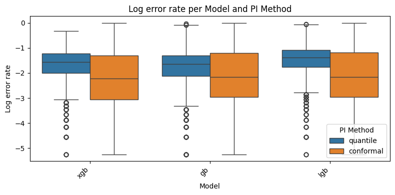
df = pd.read_csv("2024_10_22_m5_sales_uncertainty_prediction_results_local.csv")
df['log_error_rate'] = np.log(1 - df['coverage'])
df['log_winkler'] = np.log(df['winkler'])
df['log_time'] = np.log(df['time'])
df_grouped = df.groupby(['model', 'pi_method'])[['coverage', 'winkler', 'time']].agg(['min', 'median', 'max'])

df_grouped.transpose()
| model | gb | lgb | xgb | ||||
|---|---|---|---|---|---|---|---|
| pi_method | conformal | quantile | conformal | quantile | conformal | quantile | |
| coverage | min | 0.00 | 0.03 | 0.00 | 0.05 | 0.00 | 0.29 |
| median | 0.89 | 0.81 | 0.89 | 0.75 | 0.90 | 0.79 | |
| max | 1.00 | 1.00 | 1.00 | 1.00 | 1.00 | 1.00 | |
| winkler | min | 2.08 | 2.08 | 5.77 | 5.00 | 5.54 | 4.78 |
| median | 35.66 | 34.44 | 36.00 | 42.34 | 35.43 | 38.08 | |
| max | 1781.88 | 7270.32 | 1272.90 | 1304.69 | 1781.88 | 1553.96 | |
| time | min | 2.45 | 0.78 | 2.46 | 0.30 | 2.30 | 0.12 |
| median | 12.66 | 1.23 | 15.13 | 3.10 | 12.59 | 0.22 | |
| max | 152.02 | 13.71 | 149.08 | 130.01 | 63.82 | 7.96 | |
latex_table = df_grouped.transpose().applymap(lambda x: f"{x:.2f}" if isinstance(x, float) else x).to_latex()
print(latex_table)
\begin{tabular}{llllllll}
\toprule
 & model & \multicolumn{2}{r}{gb} & \multicolumn{2}{r}{lgb} & \multicolumn{2}{r}{xgb} \\
 & pi_method & conformal & quantile & conformal & quantile & conformal & quantile \\
\midrule
\multirow[t]{3}{*}{coverage} & min & 0.00 & 0.03 & 0.00 & 0.05 & 0.00 & 0.29 \\
 & median & 0.89 & 0.81 & 0.89 & 0.75 & 0.90 & 0.79 \\
 & max & 1.00 & 1.00 & 1.00 & 1.00 & 1.00 & 1.00 \\
\cline{1-8}
\multirow[t]{3}{*}{winkler} & min & 2.08 & 2.08 & 5.77 & 5.00 & 5.54 & 4.78 \\
 & median & 35.66 & 34.44 & 36.00 & 42.34 & 35.43 & 38.08 \\
 & max & 1781.88 & 7270.32 & 1272.90 & 1304.69 & 1781.88 & 1553.96 \\
\cline{1-8}
\multirow[t]{3}{*}{time} & min & 2.45 & 0.78 & 2.46 & 0.30 & 2.30 & 0.12 \\
 & median & 12.66 & 1.23 & 15.13 & 3.10 & 12.59 & 0.22 \\
 & max & 152.02 & 13.71 & 149.08 & 130.01 & 63.82 & 7.96 \\
\cline{1-8}
\bottomrule
\end{tabular}
!pip install matplotlib seaborn
import matplotlib.pyplot as plt
import seaborn as sns

# Coverage plot
plt.figure(figsize=(8, 4))
sns.boxplot(x='model', y='log_error_rate', hue='pi_method', data=df)
plt.title('Log error rate per Model and PI Method')
plt.xlabel('Model')
plt.ylabel('Log error rate')
plt.xticks(rotation=45, ha='right')
plt.legend(title='PI Method')
plt.tight_layout()
plt.show()

# Winkler plot
plt.figure(figsize=(8, 4))
sns.boxplot(x='model', y='log_winkler', hue='pi_method', data=df)
plt.title('Log Winkler Score per Model and PI Method')
plt.xlabel('Model')
plt.ylabel('Log Winkler Score')
plt.xticks(rotation=45, ha='right')
plt.legend(title='PI Method')
plt.tight_layout()
plt.show()

# Time plot
plt.figure(figsize=(8, 4))
sns.boxplot(x='model', y='log_time', hue='pi_method', data=df)
plt.title('Time per Model and PI Method')
plt.xlabel('Model')
plt.ylabel('Log Time in Log(seconds)')
plt.xticks(rotation=45, ha='right')
plt.legend(title='PI Method')
plt.tight_layout()
plt.show()

Conformalizing requires splitting the data and fitting twice, so is logically slower.
3 - 250 various time series (210 real-world, 40 synthetic)
250 time series, 240 real-world, 10 synthetic. See https://github.com/Techtonique/datasets/blob/main/time_series/univariate/250datasets/250timeseries.txt for the list of time series, and https://github.com/Techtonique/datasets/blob/main/time_series/univariate/250datasets/250datasets_characteristics.R for their characteristics.
!pip install rpy2
%load_ext rpy2.ipython
%%R

utils::install.packages(c('forecast', 'fpp', 'fpp2', 'remotes'))
remotes::install_github("Techtonique/ahead")
remotes::install_github("thierrymoudiki/simulatetimeseries")
## ----"6-twofiftydatasets", echo=FALSE, cache=TRUE, message=FALSE, warning=FALSE-------------------------------------

utils::install.packages(c("astsa",
 "datasets",
 "expsmooth",
 "fma",
 "forecast",
 "fpp",
 "fpp2",
 "MASS",
 "remotes",
 "reshape2",
 "tswge"), repos="https://cran.r-project.org", quiet=TRUE)
remotes::install_github("thierrymoudiki/simulatetimeseries")
remotes::install_github("herbps10/AdaptiveConformal")
remotes::install_github("Techtonique/ahead")

install.packages("foreach", repos="https://cran.r-project.org")
install.packages("forecast", repos="https://cran.r-project.org")


suppressWarnings(library(datasets))
suppressWarnings(library(forecast))
suppressWarnings(library(fpp2))
suppressWarnings(library(ahead))
suppressWarnings(library(simulatetimeseries))


## ----"1-foursynthplot", echo=FALSE, cache=TRUE, message=FALSE, warning=FALSE, fig.cap="4 synthetic data sets (among 47)"----
suppressWarnings(library(datasets))
suppressWarnings(library(forecast))
suppressWarnings(library(fpp2))
suppressWarnings(library(ahead))
suppressWarnings(library(simulatetimeseries))
%%R

# /!\ Despite package name, these are mostly real-world time series (210), differenced once
# (see https://github.com/Techtonique/datasets/blob/main/time_series/univariate/250datasets/250timeseries.txt)
all_datasets <- simulatetimeseries::get_data_1() # easier is to download https://github.com/Techtonique/datasets/blob/main/time_series/univariate/250datasets/all_datasets.rds

row_names <- names(all_datasets)
visualizing a few examples among the 250 time series
%%R

print(length(all_datasets))
par(mfrow=c(2, 2))
plot(all_datasets[[1]])
plot(all_datasets[[10]])
plot(all_datasets[[5]])
plot(all_datasets[[50]])
[1] 250

%%R

par(mfrow=c(2, 2))
plot(all_datasets[[2]])
plot(all_datasets[[11]])
plot(all_datasets[[9]])
plot(all_datasets[[51]])

%%R

# EXAMPLE ON A DATA SET CONTAINING 250 TIME SERIES ------------------------------------------------------------
col_names <- c("thetaf_0", "dynrmf_0",
               "thetaf_kde", "dynrmf_kde",
               "thetaf_boot", "dynrmf_boot",
               "thetaf_surr", "dynrmf_surr")

n_datasets <- length(all_datasets)
n_methods <- length(col_names)
results_winkler_score <- results_coverage_rate <- matrix(0, nrow=n_datasets, ncol=n_methods)

rownames(results_winkler_score) <- row_names
colnames(results_winkler_score) <- col_names
rownames(results_coverage_rate) <- row_names
colnames(results_coverage_rate) <- col_names

results_winkler_score <- as.data.frame(results_winkler_score)
results_coverage_rate <- as.data.frame(results_coverage_rate)

params <- vector("list", n_methods)
names(params) <- col_names

level <- 95
pct_train <- 0.9
pct_calibration <- 0.5

types_sim <- c("kde", "boot", "surr")

library("foreach")

pb <- txtProgressBar(min = 0,
                      max = n_datasets,
                      style = 3)
progress <- function(n)
  utils::setTxtProgressBar(pb, n)
opts <- list(progress = progress)
| | 0%
%%R

idx_dataset <- NULL
pb <- utils::txtProgressBar(min = 0, max = n_datasets, style = 3)

for(idx_dataset in 1:n_datasets) {

  selected_data <- all_datasets[[idx_dataset]]
  # no conformalization
  fit_obj <- try(ahead::fitforecast(selected_data, conformalize = 0, pct_train = pct_train,
                          pct_calibration=pct_calibration,
                          method = "dynrmf"), silent = TRUE)
  if (!inherits(fit_obj, "try-error"))
  {
  results_winkler_score[, "dynrmf_0"][idx_dataset] <- fit_obj$winkler_score
  results_coverage_rate[, "dynrmf_0"][idx_dataset] <- fit_obj$coverage
  } else {
    results_winkler_score[, "dynrmf_0"][idx_dataset] <- NA
    results_coverage_rate[, "dynrmf_0"][idx_dataset] <- NA
  }

  fit_obj <- try(ahead::fitforecast(selected_data, conformalize = 0, pct_train = pct_train,
                          pct_calibration=pct_calibration,
                          method = "thetaf"), silent = TRUE)
  if (!inherits(fit_obj, "try-error"))
  {
  results_winkler_score[, "thetaf_0"][idx_dataset] <- fit_obj$winkler_score
  results_coverage_rate[, "thetaf_0"][idx_dataset] <- fit_obj$coverage
  } else {
    results_winkler_score[, "thetaf_0"][idx_dataset] <- NA
    results_coverage_rate[, "thetaf_0"][idx_dataset] <- NA
  }

  # conformalization
  for (type_sim in types_sim){
    fit_obj <- try(ahead::fitforecast(selected_data, conformalize = 1,
                            pct_train = pct_train,
                            pct_calibration=pct_calibration,
                            method = "dynrmf", type_sim = type_sim), silent = TRUE)
    if (!inherits(fit_obj, "try-error"))
  {
    results_winkler_score[, paste0('dynrmf', '_', type_sim)][idx_dataset] <- fit_obj$winkler_score
    results_coverage_rate[, paste0('dynrmf', '_', type_sim)][idx_dataset] <- fit_obj$coverage #abs(fit_obj$coverage/level - 1)*100
    } else {
      results_winkler_score[, paste0('dynrmf', '_', type_sim)][idx_dataset] <- NA
      results_coverage_rate[, paste0('dynrmf', '_', type_sim)][idx_dataset] <- NA
    }

    fit_obj <- try(ahead::fitforecast(selected_data, conformalize = 1,
                            pct_train = pct_train,
                            pct_calibration=pct_calibration,
                            method = "thetaf", type_sim = type_sim), silent = TRUE)
    if (!inherits(fit_obj, "try-error"))
  {
    results_winkler_score[, paste0('thetaf', '_', type_sim)][idx_dataset] <- fit_obj$winkler_score
    results_coverage_rate[, paste0('thetaf', '_', type_sim)][idx_dataset] <- fit_obj$coverage #abs(fit_obj$coverage/level - 1)*100
    } else {
    results_winkler_score[, paste0('thetaf', '_', type_sim)][idx_dataset] <- NA
    results_coverage_rate[, paste0('thetaf', '_', type_sim)][idx_dataset] <- NA
  }

    }
    utils::setTxtProgressBar(pb, idx_dataset)
}

close(pb)
saveRDS(object = results_winkler_score, file = "results_winkler_score.rds")
saveRDS(object = results_coverage_rate, file = "results_coverage_rate.rds")
|======================================================================| 100%
De plus : Il y a eu 50 avis ou plus (utilisez warnings() pour voir les 50 premiers)
%%R

# Expected coverage rate: 95%
# methods ending with "_0" are not conformalized
# all the other methods are conformalized
coverage_ci <- t(apply(results_coverage_rate, 2, function(x) c(mean(x, na.rm = TRUE),
quantile(x, c(0.025, 0.975), na.rm = TRUE))))
colnames(coverage_ci) <- c("mean", "lower", "upper")
coverage_ci <- as.data.frame(coverage_ci)
coverage_ci$method <- rownames(coverage_ci)
coverage_ci
                mean    lower upper      method
thetaf_0    88.83283 31.57895   100    thetaf_0
dynrmf_0    87.69836 34.27419   100    dynrmf_0
thetaf_kde  88.22848 28.38095   100  thetaf_kde
dynrmf_kde  93.77326 63.22967   100  dynrmf_kde
thetaf_boot 82.48538 15.77303   100 thetaf_boot
dynrmf_boot 89.86451 33.33333   100 dynrmf_boot
thetaf_surr 84.88912 26.66667   100 thetaf_surr
dynrmf_surr 91.56125 56.22222   100 dynrmf_surr
%%R

# Winkler score, the lower the better
# methods ending with "_0" are not conformalized
# all the other methods are conformalized
winkler_ci <- t(apply(results_winkler_score, 2, function(x) c(mean(x, na.rm = TRUE),
quantile(x, c(0.025, 0.975), na.rm = TRUE))))
colnames(winkler_ci) <- c("mean", "lower", "upper")
winkler_ci <- as.data.frame(winkler_ci)
winkler_ci$method <- rownames(winkler_ci)
winkler_ci
                mean     lower     upper      method
thetaf_0    49775.61 0.3749945 150265.61    thetaf_0
dynrmf_0    21427.87 0.3624831  70254.36    dynrmf_0
thetaf_kde  45347.61 0.3803968 144066.16  thetaf_kde
dynrmf_kde  20929.91 0.3775642  62999.15  dynrmf_kde
thetaf_boot 48121.65 0.3480542 144554.24 thetaf_boot
dynrmf_boot 22728.10 0.3433424  61013.21 dynrmf_boot
thetaf_surr 48790.68 0.3499667 144421.17 thetaf_surr
dynrmf_surr 22467.88 0.3436461  61741.29 dynrmf_surr
4 - Synthetic data (25 time series)
%%R

# EXAMPLE ON A SYNTHETIC DATA SET ------------------------------------------------------------
## ----echo=FALSE, cache=FALSE, message=FALSE, warning=FALSE----------------------------------------------------------
winkler_score <- function(obj, actual, level = 95) {
  alpha <- 1 - level / 100
  lt <- obj$lower
  ut <- obj$upper
  n_points <- length(actual)
  stopifnot((n_points == length(lt)) && (n_points == length(ut)))
  diff_lt <- lt - actual
  diff_bounds <- ut - lt
  diff_ut <- actual - ut
  score <-
    diff_bounds + (2 / alpha) * (pmax(diff_lt, 0) + pmax(diff_ut, 0))
  return(mean(score))
}


## ----"7-aci-agci", echo=FALSE, cache=TRUE, message=FALSE, warning=FALSE---------------------------------------------
library("AdaptiveConformal")
library("ahead")
library("simulatetimeseries")
library("foreach")
library("forecast")

B <- 100
params_psi <- params_theta <- c(0.1, 0.8, 0.9, 0.95, 0.99)
levels <- c(80, 95)
fcast_methods <- c("thetaf", "dynrmf")
conformal_methods <- c("splitconformal", "AgACI", "SAOCP", "SF-OGD")

(params_grid <- expand.grid(params_psi, params_theta,
                            levels, fcast_methods,
                            conformal_methods))
colnames(params_grid) <- c("psi", "theta",
                           "level",
                           "fcast_method",
                           "conformal_method")
params_grid$fcast_method <- as.vector(params_grid$fcast_method)
params_grid$conformal_method <- as.vector(params_grid$conformal_method)

results <- matrix(0, ncol=B, nrow=nrow(params_grid))
colnames(results) <- paste0("B", seq_len(B))

params_grid <- params_grid2 <- cbind.data.frame(params_grid, results)

nb_iter <- nrow(params_grid)

pb <- txtProgressBar(min = 0,
                     max = nb_iter,
                     style = 3)

for (i in 1:nrow(params_grid))
{
  for (j in 6:ncol(params_grid))
  {
    seed_i_j <- 100*i+300*j

    y <- simulatetimeseries::simulate_time_series_4(n = 600,
                                                    params_grid$psi[i],
                                                    params_grid$theta[i],
                                                    seed=seed_i_j)
    splitted_ts <- simulatetimeseries::splitts(y = y, split_prob = 0.9)
    y_train <- splitted_ts$training
    y_test <- splitted_ts$testing

    if (as.character(params_grid$conformal_method[i]) == "splitconformal")
    {
      obj <- ahead::fitforecast(y,
                                conformalize = TRUE,
                                pct_train = 0.9,
                                pct_calibration = 0.5,
                                method = as.character(params_grid$fcast_method[i]),
                                type_calibration = "splitconformal",
                                level = params_grid$level[i],
                                type_sim = "kde",
                                graph = FALSE
      )
      params_grid[i, j] <- obj$coverage
      params_grid2[i, j] <- obj$winkler_score
    }

    if (as.character(params_grid$conformal_method[i]) %in% c("AgACI", "SAOCP", "SF-OGD"))
    {
      obj <- switch(as.character(params_grid$fcast_method[i]),
                      thetaf = forecast::thetaf(y_train, h=length(y_test)),
                      dynrmf = ahead::dynrmf(y_train, h=length(y_test)))
      preds <- obj$mean
      result <- AdaptiveConformal::aci(as.vector(y_test),
                                       as.vector(preds),
                                       method = as.character(params_grid$conformal_method[i]),
                                       alpha = params_grid$level[i]/100)
      result$lower <- result$intervals[, 1]
      result$upper <- result$intervals[, 2]
      params_grid[i, j] <- result$metrics$coverage*100
      params_grid2[i, j] <- winkler_score(result, actual=y_test, level = params_grid$level[i])
    }
  }
  utils::setTxtProgressBar(pb, i)
}

close(pb)

saveRDS(params_grid, "params_grid_coverages.rds")
saveRDS(params_grid2, "params_grid_winkler.rds")
4 - 1 Coverage rates for synthetic data
%%R

# CONFIDENCE INTERVALS FOR THE SYNTHETIC DATA SET
## ----"11-ag-agci-confint-coverage", echo=FALSE, cache=TRUE, warning=FALSE, message=FALSE----------------------------
utils::install.packages("dplyr", repos = "https://cran.r-project.org")
library("dplyr")
df <- reshape2::melt(params_grid,
                          id.vars=c("level",
                           "fcast_method",
                           "conformal_method"),
                          measure.vars=paste0("B", seq_len(B)))
df$variable <- NULL
%%R

utils::install.packages("patchwork")
library(patchwork)
%%R

# Create interaction label for x-axis
df$method_combo <- paste(df$fcast_method, df$conformal_method, sep="\n")

# Summary tables for each level
table_80 <- df %>%
  filter(level == 80) %>%
  group_by(fcast_method, conformal_method) %>%
  summarise(
    mean = mean(value),
    sd = sd(value),
    median = median(value),
    q25 = quantile(value, 0.25),
    q75 = quantile(value, 0.75)
  ) %>%
  arrange(desc(mean))

table_95 <- df %>%
  filter(level == 95) %>%
  group_by(fcast_method, conformal_method) %>%
  summarise(
    mean = mean(value),
    sd = sd(value),
    median = median(value),
    q25 = quantile(value, 0.25),
    q75 = quantile(value, 0.75)
  ) %>%
  arrange(desc(mean))

# Plot for level 80
p1 <- ggplot(df[df$level == 80,], aes(x=method_combo, y=value)) +
  geom_boxplot(fill="lightgray") +
  labs(title="Distribution of Coverage Rates by Method (Level = 80)",
       x="Forecasting Method + Conformal Method",
       y="Value") +
  theme_minimal() +
  theme(axis.text.x = element_text(angle = 45, hjust = 1))

# Plot for level 95
p2 <- ggplot(df[df$level == 95,], aes(x=method_combo, y=value)) +
  geom_boxplot(fill="lightgray") +
  labs(title="Distribution of Coverage Rates by Method (Level = 95)",
       x="Forecasting Method + Conformal Method",
       y="Value") +
  theme_minimal() +
  theme(axis.text.x = element_text(angle = 45, hjust = 1))

# Display plots one after another using patchwork
library(patchwork)
print(p1 / p2)
`summarise()` has grouped output by 'fcast_method'. You can override using the
`.groups` argument.
`summarise()` has grouped output by 'fcast_method'. You can override using the
`.groups` argument.

%%R

# Print formatted tables
cat("Coverage Rate Summary Statistics for Level 80:\n")
print(kable(table_80, digits = 2))
Coverage Rate Summary Statistics for Level 80:


|fcast_method |conformal_method |  mean|   sd| median|   q25|   q75|
|:------------|:----------------|-----:|----:|------:|-----:|-----:|
|dynrmf       |splitconformal   | 81.40| 7.37|  83.33| 76.67| 86.67|
|thetaf       |splitconformal   | 79.85| 8.50|  81.67| 75.00| 85.00|
|dynrmf       |AgACI            | 77.61| 4.06|  78.33| 75.00| 80.00|
|thetaf       |AgACI            | 77.41| 4.08|  78.33| 75.00| 80.00|
|dynrmf       |SAOCP            | 52.77| 3.76|  53.33| 50.00| 55.00|
|thetaf       |SAOCP            | 51.81| 4.73|  51.67| 50.00| 55.00|
|dynrmf       |SF-OGD           |  1.20| 1.39|   1.67|  0.00|  1.67|
|thetaf       |SF-OGD           |  1.16| 1.38|   0.00|  0.00|  1.67|
%%R

cat("\nCoverage Rate Summary Statistics for Level 95:\n")
print(kable(table_95, digits = 2))
Coverage Rate Summary Statistics for Level 95:


|fcast_method |conformal_method |  mean|   sd| median|   q25|   q75|
|:------------|:----------------|-----:|----:|------:|-----:|-----:|
|dynrmf       |splitconformal   | 95.57| 4.12|  96.67| 93.33| 98.33|
|thetaf       |splitconformal   | 94.38| 4.96|  95.00| 91.67| 98.33|
|dynrmf       |AgACI            | 89.98| 3.02|  90.00| 88.33| 91.67|
|thetaf       |AgACI            | 89.74| 3.12|  90.00| 88.33| 91.67|
|dynrmf       |SAOCP            | 59.56| 3.85|  60.00| 56.67| 61.67|
|thetaf       |SAOCP            | 58.41| 4.91|  58.33| 56.67| 61.67|
|dynrmf       |SF-OGD           |  1.19| 1.39|   1.67|  0.00|  1.67|
|thetaf       |SF-OGD           |  1.17| 1.37|   1.67|  0.00|  1.67|
4 - 2 Winkler scores for synthetic data
The lower the better.
%%R

## ----"12-ag-agci-confint-winkler", echo=FALSE, cache=TRUE, warning=FALSE, message=FALSE-----------------------------
df <- reshape2::melt(params_grid2,
                          id.vars=c("level",
                           "fcast_method",
                           "conformal_method"),
                          measure.vars=paste0("B", seq_len(B)))
df$variable <- NULL
%%R

# Create interaction label for x-axis
df$method_combo <- paste(df$fcast_method, df$conformal_method, sep="\n")

# Summary tables for each level
table_80 <- df %>%
  filter(level == 80) %>%
  group_by(fcast_method, conformal_method) %>%
  summarise(
    mean = mean(value),
    sd = sd(value),
    median = median(value),
    q25 = quantile(value, 0.25),
    q75 = quantile(value, 0.75)
  ) %>%
  arrange(desc(mean))

table_95 <- df %>%
  filter(level == 95) %>%
  group_by(fcast_method, conformal_method) %>%
  summarise(
    mean = mean(value),
    sd = sd(value),
    median = median(value),
    q25 = quantile(value, 0.25),
    q75 = quantile(value, 0.75)
  ) %>%
  arrange(desc(mean))

# Plot for level 80
p1 <- ggplot(df[df$level == 80,], aes(x=method_combo, y=value)) +
  geom_boxplot(fill="lightgray") +
  labs(title="Distribution of Winkler Scores by Method (Level = 80)",
       x="Forecasting Method + Conformal Method",
       y="Value") +
  theme_minimal() +
  theme(axis.text.x = element_text(angle = 45, hjust = 1))

# Plot for level 95
p2 <- ggplot(df[df$level == 95,], aes(x=method_combo, y=value)) +
  geom_boxplot(fill="lightgray") +
  labs(title="Distribution of Winkler Scores by Method (Level = 95)",
       x="Forecasting Method + Conformal Method",
       y="Value") +
  theme_minimal() +
  theme(axis.text.x = element_text(angle = 45, hjust = 1))

# Display plots one after another using patchwork
library(patchwork)
print(p1 / p2)
`summarise()` has grouped output by 'fcast_method'. You can override using the
`.groups` argument.
`summarise()` has grouped output by 'fcast_method'. You can override using the
`.groups` argument.

%%R

# Print formatted tables
cat("Winkler Score Summary Statistics for Level 80:\n")
print(kable(table_80, digits = 2))
Winkler Score Summary Statistics for Level 80:


|fcast_method |conformal_method |  mean|   sd| median|   q25|   q75|
|:------------|:----------------|-----:|----:|------:|-----:|-----:|
|thetaf       |SF-OGD           | 47.91| 8.74|  46.39| 42.21| 51.26|
|dynrmf       |SF-OGD           | 46.16| 6.03|  45.57| 42.16| 49.59|
|thetaf       |SAOCP            | 26.23| 5.01|  25.33| 22.90| 28.45|
|dynrmf       |SAOCP            | 24.95| 3.59|  24.61| 22.47| 26.83|
|thetaf       |AgACI            | 21.85| 3.10|  21.53| 19.58| 23.52|
|thetaf       |splitconformal   | 21.16| 3.79|  20.41| 18.82| 22.50|
|dynrmf       |AgACI            | 21.07| 2.49|  20.87| 19.37| 22.55|
|dynrmf       |splitconformal   | 20.28| 2.85|  19.78| 18.53| 21.44|
%%R

# Print formatted tables
# Winkler score, the lower the better
cat("Winkler Score Summary Statistics for Level 95:\n")
print(kable(table_95, digits = 2))
Winkler Score Summary Statistics for Level 95:


|fcast_method |conformal_method |   mean|    sd| median|    q25|    q75|
|:------------|:----------------|------:|-----:|------:|------:|------:|
|thetaf       |SF-OGD           | 191.33| 33.69| 185.45| 169.11| 205.35|
|dynrmf       |SF-OGD           | 183.80| 23.78| 181.53| 168.26| 197.23|
|thetaf       |SAOCP            |  67.82| 16.35|  65.02|  56.87|  74.78|
|dynrmf       |SAOCP            |  63.90| 11.80|  62.66|  55.78|  70.58|
|thetaf       |AgACI            |  32.80|  4.95|  32.20|  29.26|  35.67|
|dynrmf       |AgACI            |  31.82|  4.15|  31.53|  28.83|  34.36|
|thetaf       |splitconformal   |  28.01|  6.01|  26.39|  24.51|  29.46|
|dynrmf       |splitconformal   |  26.56|  4.68|  25.63|  24.05|  27.89|
5 - Session info
5 - 1 Python
import platform

# Get basic machine information
python_version = platform.python_version()

print("Python Version:", python_version)
Python Version: 3.11.10
import psutil

# CPU Information
cpu_count = psutil.cpu_count(logical=True)
cpu_freq = psutil.cpu_freq()
cpu_usage = psutil.cpu_percent(interval=1)

# Memory Information
virtual_memory = psutil.virtual_memory()
swap_memory = psutil.swap_memory()

# Disk Information
disk_usage = psutil.disk_usage('/')

print(f"CPU Count: {cpu_count}")
print(f"CPU Frequency: {cpu_freq.current} MHz")
CPU Count: 8
CPU Frequency: 1100 MHz
!pip freeze
Python(54508) MallocStackLogging: can't turn off malloc stack logging because it was not enabled.
appnope==0.1.4
asttokens==2.4.1
certifi==2024.12.14
cffi==1.17.1
charset-normalizer==3.4.1
click==8.1.7
comm==0.2.1
contourpy==1.3.1
cycler==0.12.1
debugpy==1.8.1
decorator==5.1.1
executing==2.0.1
fonttools==4.55.3
idna==3.10
ipykernel==6.29.3
ipython==8.22.2
jedi==0.19.1
Jinja2==3.1.5
joblib==1.4.2
jupyter_client==8.6.0
jupyter_core==5.7.1
kiwisolver==1.4.8
lightgbm==4.5.0
MarkupSafe==3.0.2
matplotlib==3.10.0
matplotlib-inline==0.1.6
nest-asyncio==1.6.0
nnetsauce==0.29.5
numpy==2.2.1
packaging==23.2
pandas==2.2.3
parso==0.8.3
patsy==1.0.1
pexpect==4.9.0
pillow==11.1.0
platformdirs==4.2.0
prompt-toolkit==3.0.43
psutil==5.9.8
ptyprocess==0.7.0
pure-eval==0.2.2
pycparser==2.22
Pygments==2.17.2
pyparsing==3.2.1
python-dateutil==2.9.0.post0
pytz==2024.2
pyzmq==25.1.2
requests==2.32.3
rpy2==3.5.17
rtopy==0.1.1
scikit-learn==1.6.0
scipy==1.15.0
seaborn==0.13.2
six==1.16.0
stack-data==0.6.3
statsmodels==0.14.4
threadpoolctl==3.5.0
tornado==6.4
tqdm==4.67.1
traitlets==5.14.1
tzdata==2024.2
tzlocal==5.2
urllib3==2.3.0
wcwidth==0.2.13
xgboost==2.1.3
5 - 2 R
%R sessionInfo()
| R.version |
ListVector with 14 elements.
|
||||||||||||||||||||
|---|---|---|---|---|---|---|---|---|---|---|---|---|---|---|---|---|---|---|---|---|---|
| platform |
StrVector with 1 elements.
|
||||||||||||||||||||
| locale |
StrVector with 1 elements.
|
||||||||||||||||||||
| ... | ... | ||||||||||||||||||||
| BLAS |
StrVector with 1 elements.
|
||||||||||||||||||||
| LAPACK |
StrVector with 1 elements.
|
||||||||||||||||||||
| LA_version |
StrVector with 1 elements.
|
Conclusion
So, based on these extensive experiments against the state of the art (and assuming the implementations of the state of the art methods are correct, which I’m sure they are, see https://computo.sfds.asso.fr/published-202407-susmann-adaptive-conformal/, and assuming I’m using them well), how cool is this contribution to the science of forecasting? My results are particularly impressive on the 3003 time series from the M3 competition (versus other quite recent conformal prediction methods). On M5 competition data, the method is performing on par with XGBoost, LightGBM, GradientBoostingRegressor quantile regressors. All from 3 prominent package heavyweights on the market. My 2 cents (but I might be wrong): almost nobody likes simplicity in corporate world, and in academia in particular, because they need to justify, somehow, why something is expensive/why they are funded. A bias that fuels complexity (read: complex=”substantial”) for the sake of complexity. Man, IT JUST WORKS. And even more than that, as hopefully demonstrated here with extensive benchmarks.
For attribution, please cite this work as:
T. Moudiki (2025-01-05). Just got a paper on conformal prediction REJECTED by International Journal of Forecasting despite evidence on 30,000 time series (and more). What's going on?. Retrieved from https://thierrymoudiki.github.io/blog/2025/01/05/r/forecasting/python/misc/ijf-benchmark-rejection
BibTeX citation (remove empty spaces)
        @misc{ tmoudiki20250105,
          author = { T. Moudiki },
          title = { Just got a paper on conformal prediction REJECTED by International Journal of Forecasting despite evidence on 30,000 time series (and more). What's going on? },
          url = { https://thierrymoudiki.github.io/blog/2025/01/05/r/forecasting/python/misc/ijf-benchmark-rejection },
          year = { 2025 } }

Previous publications
- GPopt for R: Bayesian and conformal optimization of black-box functions and hyperparameter tuning Jul 26, 2026
- My last R posts: How conformalization helps weak models, fast conformal prediction with jackknife+ (and no refitting), and sklearn in R Jul 13, 2026
- Natively Interpretable Boosting Jul 12, 2026
- Fast conformal prediction (no refitting) for some Machine Learning models via closed-form jackknife plus Jun 27, 2026
- Using scikit-learn models in R easily with the tisthemachinelearner package Jun 21, 2026
- No-Code Machine Learning in Excel with the Techtonique API Jun 14, 2026
- How Conformal Prediction Makes Linear Models Good Enough — An Example Using R Package mlS3 Jun 7, 2026
- Techtonique dot net, the Machine Learning web API, is back online (but more like a passion project for now) May 31, 2026
- Conformalized TabICL: Prediction Intervals for a State-Of-The-Art Tabular Foundation Model in Python and R May 21, 2026
- Conformalized TabPFN: Prediction Intervals for a Pretrained Transformer for Tabular Data in Python and R May 17, 2026
- Probabilistic Time Series Cross-Validation with R package crossvalidation May 16, 2026
- One interface, (Almost) Every Classifier (and Regressor): unifiedml v0.3.0 May 9, 2026
- You Don't Need to Learn All the Weights on tabular data: The Case for rvflnet (a nonlinear expressive glmnet) on regression, classification and survival analysis May 2, 2026
- Survival analysis with sklearn, glmnet, keras, pytorch, lightgbm, xgboost, nnetsauce, mlsauce Part 2 Apr 28, 2026
- Any Sklearn Regressor as a Survival Model — Does It Actually Work? Benchmarking vs Established Packages Apr 26, 2026
- Conformal Optimization Beats Bayesian Optimization, Optuna and Random Search on 72 classification Datasets Apr 19, 2026
- `mlS3` — A Unified S3 Machine Learning Interface in R Apr 12, 2026
- One interface, (Almost) Every Classifier: unifiedml v0.2.1 Apr 4, 2026
- Techtonique dot net is down until further notice Apr 1, 2026
- Explaining Time-Series Forecasts with Sensitivity Analysis (ahead::dynrmf and external regressors) Mar 29, 2026
- Python version of 'Option pricing using time series models as market price of risk Pt.3' Mar 22, 2026
- Option pricing using time series models as market price of risk Pt.3 Mar 16, 2026
- Explaining Time-Series Forecasts with Exact Shapley Values (ahead::dynrmf with external regressors applied to scenarios) Mar 8, 2026
- My Presentation at Risk 2026: Lightweight Transfer Learning for Financial Forecasting Mar 1, 2026
- nnetsauce with and without jax for GPU acceleration Feb 23, 2026
- Understanding Boosted Configuration Networks (combined neural networks and boosting): An Intuitive Guide Through Their Hyperparameters Feb 16, 2026
- R version of Python package survivalist, for model-agnostic survival analysis Feb 9, 2026
- Presenting Lightweight Transfer Learning for Financial Forecasting (Risk 2026) Feb 4, 2026
- Option pricing using time series models as market price of risk Feb 1, 2026
- Enhancing Time Series Forecasting (ahead::ridge2f) with Attention-Based Context Vectors (ahead::contextridge2f) Jan 31, 2026
- Overfitting and scaling (on GPU T4) tests on nnetsauce.CustomRegressor Jan 29, 2026
- Beyond Cross-validation: Hyperparameter Optimization via Generalization Gap Modeling Jan 25, 2026
- GPopt for Machine Learning (hyperparameters' tuning) Jan 21, 2026
- rtopy: an R to Python bridge -- novelties Jan 8, 2026
- Python examples for 'Beyond Nelson-Siegel and splines: A model- agnostic Machine Learning framework for discount curve calibration, interpolation and extrapolation' Jan 3, 2026
- Forecasting benchmark: Dynrmf (a new serious competitor in town) vs Theta Method on M-Competitions and Tourism competitition Jan 1, 2026
- Finally figured out a way to port python packages to R using uv and reticulate: example with nnetsauce Dec 17, 2025
- Overfitting Random Fourier Features: Universal Approximation Property Dec 13, 2025
- Counterfactual Scenario Analysis with ahead::ridge2f Dec 11, 2025
- Zero-Shot Probabilistic Time Series Forecasting with TabPFN 2.5 and nnetsauce Dec 10, 2025
- ARIMA Pricing: Semi-Parametric Market price of risk for Risk-Neutral Pricing (code + preprint) Dec 7, 2025
- Analyzing Paper Reviews with LLMs: I Used ChatGPT, DeepSeek, Qwen, Mistral, Gemini, and Claude (and you should too + publish the analysis) Dec 3, 2025
- tisthemachinelearner: New Workflow with uv for R Integration of scikit-learn Dec 1, 2025
- (ICYMI) RPweave: Unified R + Python + LaTeX System using uv Nov 21, 2025
- unifiedml: A Unified Machine Learning Interface for R, is now on CRAN + Discussion about AI replacing humans Nov 16, 2025
- Context-aware Theta forecasting Method: Extending Classical Time Series Forecasting with Machine Learning Nov 13, 2025
- unifiedml in R: A Unified Machine Learning Interface Nov 5, 2025
- Deterministic Shift Adjustment in Arbitrage-Free Pricing (historical to risk-neutral short rates) Oct 28, 2025
- New instantaneous short rates models with their deterministic shift adjustment, for historical and risk-neutral simulation Oct 27, 2025
- RPweave: Unified R + Python + LaTeX System using uv Oct 19, 2025
- GAN-like Synthetic Data Generation Examples (on univariate, multivariate distributions, digits recognition, Fashion-MNIST, stock returns, and Olivetti faces) with DistroSimulator Oct 19, 2025
- R port of llama2.c Oct 9, 2025
- Native uncertainty quantification for time series with NGBoost Oct 8, 2025
- NGBoost (Natural Gradient Boosting) for Regression, Classification, Time Series forecasting and Reserving Oct 6, 2025
- Real-time pricing with a pretrained probabilistic stock return model Oct 1, 2025
- Combining any model with GARCH(1,1) for probabilistic stock forecasting Sep 23, 2025
- Generating Synthetic Data with R-vine Copulas using esgtoolkit in R Sep 21, 2025
- Reimagining Equity Solvency Capital Requirement Approximation (one of my Master's Thesis subjects): From Bilinear Interpolation to Probabilistic Machine Learning Sep 16, 2025
- Transfer Learning using ahead::ridge2f on synthetic stocks returns Pt.2: synthetic data generation Sep 9, 2025
- Transfer Learning using ahead::ridge2f on synthetic stocks returns Sep 8, 2025
- I'm supposed to present 'Conformal Predictive Simulations for Univariate Time Series' at COPA CONFERENCE 2025 in London... Sep 4, 2025
- external regressors in ahead::dynrmf's interface for Machine learning forecasting Sep 1, 2025
- Another interesting decision, now for 'Beyond Nelson-Siegel and splines: A model-agnostic Machine Learning framework for discount curve calibration, interpolation and extrapolation' Aug 20, 2025
- Boosting any randomized based learner for regression, classification and univariate/multivariate time series forcasting Jul 26, 2025
- New nnetsauce version with CustomBackPropRegressor (CustomRegressor with Backpropagation) and ElasticNet2Regressor (Ridge2 with ElasticNet regularization) Jul 15, 2025
- mlsauce (home to a model-agnostic gradient boosting algorithm) can now be installed from PyPI. Jul 10, 2025
- A user-friendly graphical interface to techtonique dot net's API (will eventually contain graphics). Jul 8, 2025
- Calling =TECHTO_MLCLASSIFICATION for Machine Learning supervised CLASSIFICATION in Excel is just a matter of copying and pasting Jul 7, 2025
- Calling =TECHTO_MLREGRESSION for Machine Learning supervised regression in Excel is just a matter of copying and pasting Jul 6, 2025
- Calling =TECHTO_RESERVING and =TECHTO_MLRESERVING for claims triangle reserving in Excel is just a matter of copying and pasting Jul 5, 2025
- Calling =TECHTO_SURVIVAL for Survival Analysis in Excel is just a matter of copying and pasting Jul 4, 2025
- Calling =TECHTO_SIMULATION for Stochastic Simulation in Excel is just a matter of copying and pasting Jul 3, 2025
- Calling =TECHTO_FORECAST for forecasting in Excel is just a matter of copying and pasting Jul 2, 2025
- Random Vector Functional Link (RVFL) artificial neural network with 2 regularization parameters successfully used for forecasting/synthetic simulation in professional settings: Extensions (including Bayesian) Jul 1, 2025
- R version of 'Backpropagating quasi-randomized neural networks' Jun 24, 2025
- Backpropagating quasi-randomized neural networks Jun 23, 2025
- Beyond ARMA-GARCH: leveraging any statistical model for volatility forecasting Jun 21, 2025
- Stacked generalization (Machine Learning model stacking) + conformal prediction for forecasting with ahead::mlf Jun 18, 2025
- An Overfitting dilemma: XGBoost Default Hyperparameters vs GenericBooster + LinearRegression Default Hyperparameters Jun 14, 2025
- Programming language-agnostic reserving using RidgeCV, LightGBM, XGBoost, and ExtraTrees Machine Learning models Jun 13, 2025
- Free R, Python and SQL editors in techtonique dot net Jun 9, 2025
- Beyond Nelson-Siegel and splines: A model-agnostic Machine Learning framework for discount curve calibration, interpolation and extrapolation Jun 7, 2025
- scikit-learn, glmnet, xgboost, lightgbm, pytorch, keras, nnetsauce in probabilistic Machine Learning (for longitudinal data) Reserving (work in progress) Jun 6, 2025
- R version of Probabilistic Machine Learning (for longitudinal data) Reserving (work in progress) Jun 5, 2025
- Probabilistic Machine Learning (for longitudinal data) Reserving (work in progress) Jun 4, 2025
- Python version of Beyond ARMA-GARCH: leveraging model-agnostic Quasi-Randomized networks and conformal prediction for nonparametric probabilistic stock forecasting (ML-ARCH) Jun 3, 2025
- Beyond ARMA-GARCH: leveraging model-agnostic Machine Learning and conformal prediction for nonparametric probabilistic stock forecasting (ML-ARCH) Jun 2, 2025
- Permutations and SHAPley values for feature importance in techtonique dot net's API (with R + Python + the command line) Jun 1, 2025
- Which patient is going to survive longer? Another guide to using techtonique dot net's API (with R + Python + the command line) for survival analysis May 31, 2025
- A Guide to Using techtonique.net's API and rush for simulating and plotting Stochastic Scenarios May 30, 2025
- Simulating Stochastic Scenarios with Diffusion Models: A Guide to Using techtonique.net's API for the purpose May 29, 2025
- Will my apartment in 5th avenue be overpriced or not? Harnessing the power of www.techtonique.net (+ xgboost, lightgbm, catboost) to find out May 28, 2025
- How long must I wait until something happens: A Comprehensive Guide to Survival Analysis via an API May 27, 2025
- Harnessing the Power of techtonique.net: A Comprehensive Guide to Machine Learning Classification via an API May 26, 2025
- Quantile regression with any regressor -- Examples with RandomForestRegressor, RidgeCV, KNeighborsRegressor May 20, 2025
- Survival stacking: survival analysis translated as supervised classification in R and Python May 5, 2025
- 'Bayesian' optimization of hyperparameters in a R machine learning model using the bayesianrvfl package Apr 25, 2025
- A lightweight interface to scikit-learn in R: Bayesian and Conformal prediction Apr 21, 2025
- A lightweight interface to scikit-learn in R Pt.2: probabilistic time series forecasting in conjunction with ahead::dynrmf Apr 20, 2025
- Extending the Theta forecasting method to GLMs, GAMs, GLMBOOST and attention: benchmarking on Tourism, M1, M3 and M4 competition data sets (28000 series) Apr 14, 2025
- Extending the Theta forecasting method to GLMs and attention Apr 8, 2025
- Nonlinear conformalized Generalized Linear Models (GLMs) with R package 'rvfl' (and other models) Mar 31, 2025
- Probabilistic Time Series Forecasting (predictive simulations) in Microsoft Excel using Python, xlwings lite and www.techtonique.net Mar 28, 2025
- Conformalize (improved prediction intervals and simulations) any R Machine Learning model with misc::conformalize Mar 25, 2025
- My poster for the 18th FINANCIAL RISKS INTERNATIONAL FORUM by Institut Louis Bachelier/Fondation du Risque/Europlace Institute of Finance Mar 19, 2025
- Interpretable probabilistic kernel ridge regression using Matérn 3/2 kernels Mar 16, 2025
- (News from) Probabilistic Forecasting of univariate and multivariate Time Series using Quasi-Randomized Neural Networks (Ridge2) and Conformal Prediction Mar 9, 2025
- Word-Online: re-creating Karpathy's char-RNN (with supervised linear online learning of word embeddings) for text completion Mar 8, 2025
- CRAN-like repository for most recent releases of Techtonique's R packages Mar 2, 2025
- Presenting 'Online Probabilistic Estimation of Carbon Beta and Carbon Shapley Values for Financial and Climate Risk' at Institut Louis Bachelier Feb 27, 2025
- Web app with DeepSeek R1 and Hugging Face API for chatting Feb 23, 2025
- tisthemachinelearner: A Lightweight interface to scikit-learn with 2 classes, Classifier and Regressor (in Python and R) Feb 17, 2025
- R version of survivalist: Probabilistic model-agnostic survival analysis using scikit-learn, xgboost, lightgbm (and conformal prediction) Feb 12, 2025
- Model-agnostic global Survival Prediction of Patients with Myeloid Leukemia in QRT/Gustave Roussy Challenge (challengedata.ens.fr): Python's survivalist Quickstart Feb 10, 2025
- A simple test of the martingale hypothesis in esgtoolkit Feb 3, 2025
- Command Line Interface (CLI) for techtonique.net's API Jan 31, 2025
- Gradient-Boosting and Boostrap aggregating anything (alert: high performance): Part5, easier install and Rust backend Jan 27, 2025
- Just got a paper on conformal prediction REJECTED by International Journal of Forecasting despite evidence on 30,000 time series (and more). What's going on? Part2: 1311 time series from the Tourism competition Jan 20, 2025
- Techtonique is released! (with a tutorial in various programming languages and formats) Jan 14, 2025
- Univariate and Multivariate Probabilistic Forecasting with nnetsauce and TabPFN Jan 14, 2025
- Just got a paper on conformal prediction REJECTED by International Journal of Forecasting despite evidence on 30,000 time series (and more). What's going on? Jan 5, 2025
- Python and Interactive dashboard version of Stock price forecasting with Deep Learning: throwing power at the problem (and why it won't make you rich) Dec 31, 2024
- Stock price forecasting with Deep Learning: throwing power at the problem (and why it won't make you rich) Dec 29, 2024
- No-code Machine Learning Cross-validation and Interpretability in techtonique.net Dec 23, 2024
- survivalist: Probabilistic model-agnostic survival analysis using scikit-learn, glmnet, xgboost, lightgbm, pytorch, keras, nnetsauce and mlsauce Dec 15, 2024
- Model-agnostic 'Bayesian' optimization (for hyperparameter tuning) using conformalized surrogates in GPopt Dec 9, 2024
- You can beat Forecasting LLMs (Large Language Models a.k.a foundation models) with nnetsauce.MTS Pt.2: Generic Gradient Boosting Dec 1, 2024
- You can beat Forecasting LLMs (Large Language Models a.k.a foundation models) with nnetsauce.MTS Nov 24, 2024
- Unified interface and conformal prediction (calibrated prediction intervals) for R package forecast (and 'affiliates') Nov 23, 2024
- GLMNet in Python: Generalized Linear Models Nov 18, 2024
- Gradient-Boosting anything (alert: high performance): Part4, Time series forecasting Nov 10, 2024
- Predictive scenarios simulation in R, Python and Excel using Techtonique API Nov 3, 2024
- Chat with your tabular data in www.techtonique.net Oct 30, 2024
- Gradient-Boosting anything (alert: high performance): Part3, Histogram-based boosting Oct 28, 2024
- R editor and SQL console (in addition to Python editors) in www.techtonique.net Oct 21, 2024
- R and Python consoles + JupyterLite in www.techtonique.net Oct 15, 2024
- Gradient-Boosting anything (alert: high performance): Part2, R version Oct 14, 2024
- Gradient-Boosting anything (alert: high performance) Oct 6, 2024
- Benchmarking 30 statistical/Machine Learning models on the VN1 Forecasting -- Accuracy challenge Oct 4, 2024
- Automated random variable distribution inference using Kullback-Leibler divergence and simulating best-fitting distribution Oct 2, 2024
- Forecasting in Excel using Techtonique's Machine Learning APIs under the hood Sep 30, 2024
- Techtonique web app for data-driven decisions using Mathematics, Statistics, Machine Learning, and Data Visualization Sep 25, 2024
- Parallel for loops (Map or Reduce) + New versions of nnetsauce and ahead Sep 16, 2024
- Adaptive (online/streaming) learning with uncertainty quantification using Polyak averaging in learningmachine Sep 10, 2024
- New versions of nnetsauce and ahead Sep 9, 2024
- Prediction sets and prediction intervals for conformalized Auto XGBoost, Auto LightGBM, Auto CatBoost, Auto GradientBoosting Sep 2, 2024
- Quick/automated R package development workflow (assuming you're using macOS or Linux) Part2 Aug 30, 2024
- R package development workflow (assuming you're using macOS or Linux) Aug 27, 2024
- A new method for deriving a nonparametric confidence interval for the mean Aug 26, 2024
- Conformalized adaptive (online/streaming) learning using learningmachine in Python and R Aug 19, 2024
- Bayesian (nonlinear) adaptive learning Aug 12, 2024
- Auto XGBoost, Auto LightGBM, Auto CatBoost, Auto GradientBoosting Aug 5, 2024
- Copulas for uncertainty quantification in time series forecasting Jul 28, 2024
- Forecasting uncertainty: sequential split conformal prediction + Block bootstrap (web app) Jul 22, 2024
- learningmachine for Python (new version) Jul 15, 2024
- learningmachine v2.0.0: Machine Learning with explanations and uncertainty quantification Jul 8, 2024
- My presentation at ISF 2024 conference (slides with nnetsauce probabilistic forecasting news) Jul 3, 2024
- 10 uncertainty quantification methods in nnetsauce forecasting Jul 1, 2024
- Forecasting with XGBoost embedded in Quasi-Randomized Neural Networks Jun 24, 2024
- Forecasting Monthly Airline Passenger Numbers with Quasi-Randomized Neural Networks Jun 17, 2024
- Automated hyperparameter tuning using any conformalized surrogate Jun 9, 2024
- Recognizing handwritten digits with Ridge2Classifier Jun 3, 2024
- Forecasting the Economy May 27, 2024
- A detailed introduction to Deep Quasi-Randomized 'neural' networks May 19, 2024
- Probability of receiving a loan; using learningmachine May 12, 2024
- mlsauce's `v0.18.2`: various examples and benchmarks with dimension reduction May 6, 2024
- mlsauce's `v0.17.0`: boosting with Elastic Net, polynomials and heterogeneity in explanatory variables Apr 29, 2024
- mlsauce's `v0.13.0`: taking into account inputs heterogeneity through clustering Apr 21, 2024
- mlsauce's `v0.12.0`: prediction intervals for LSBoostRegressor Apr 15, 2024
- Conformalized predictive simulations for univariate time series on more than 250 data sets Apr 7, 2024
- learningmachine v1.1.2: for Python Apr 1, 2024
- learningmachine v1.0.0: prediction intervals around the probability of the event 'a tumor being malignant' Mar 25, 2024
- Bayesian inference and conformal prediction (prediction intervals) in nnetsauce v0.18.1 Mar 18, 2024
- Multiple examples of Machine Learning forecasting with ahead Mar 11, 2024
- rtopy (v0.1.1): calling R functions in Python Mar 4, 2024
- ahead forecasting (v0.10.0): fast time series model calibration and Python plots Feb 26, 2024
- A plethora of datasets at your fingertips Part3: how many times do couples cheat on each other? Feb 19, 2024
- nnetsauce's introduction as of 2024-02-11 (new version 0.17.0) Feb 11, 2024
- Tuning Machine Learning models with GPopt's new version Part 2 Feb 5, 2024
- Tuning Machine Learning models with GPopt's new version Jan 29, 2024
- Subsampling continuous and discrete response variables Jan 22, 2024
- DeepMTS, a Deep Learning Model for Multivariate Time Series Jan 15, 2024
- A classifier that's very accurate (and deep) Pt.2: there are > 90 classifiers in nnetsauce Jan 8, 2024
- learningmachine: prediction intervals for conformalized Kernel ridge regression and Random Forest Jan 1, 2024
- A plethora of datasets at your fingertips Part2: how many times do couples cheat on each other? Descriptive analytics, interpretability and prediction intervals using conformal prediction Dec 25, 2023
- Diffusion models in Python with esgtoolkit (Part2) Dec 18, 2023
- Diffusion models in Python with esgtoolkit Dec 11, 2023
- Julia packaging at the command line Dec 4, 2023
- Quasi-randomized nnetworks in Julia, Python and R Nov 27, 2023
- A plethora of datasets at your fingertips Nov 20, 2023
- A classifier that's very accurate (and deep) Nov 12, 2023
- mlsauce version 0.8.10: Statistical/Machine Learning with Python and R Nov 5, 2023
- AutoML in nnetsauce (randomized and quasi-randomized nnetworks) Pt.2: multivariate time series forecasting Oct 29, 2023
- AutoML in nnetsauce (randomized and quasi-randomized nnetworks) Oct 22, 2023
- Version v0.14.0 of nnetsauce for R and Python Oct 16, 2023
- A diffusion model: G2++ Oct 9, 2023
- Diffusion models in ESGtoolkit + announcements Oct 2, 2023
- An infinity of time series forecasting models in nnetsauce (Part 2 with uncertainty quantification) Sep 25, 2023
- (News from) forecasting in Python with ahead (progress bars and plots) Sep 18, 2023
- Forecasting in Python with ahead Sep 11, 2023
- Risk-neutralize simulations Sep 4, 2023
- Comparing cross-validation results using crossval_ml and boxplots Aug 27, 2023
- Reminder Apr 30, 2023
- Did you ask ChatGPT about who you are? Apr 16, 2023
- A new version of nnetsauce (randomized and quasi-randomized 'neural' networks) Apr 2, 2023
- Simple interfaces to the forecasting API Nov 23, 2022
- A web application for forecasting in Python, R, Ruby, C#, JavaScript, PHP, Go, Rust, Java, MATLAB, etc. Nov 2, 2022
- Prediction intervals (not only) for Boosted Configuration Networks in Python Oct 5, 2022
- Boosted Configuration (neural) Networks Pt. 2 Sep 3, 2022
- Boosted Configuration (_neural_) Networks for classification Jul 21, 2022
- A Machine Learning workflow using Techtonique Jun 6, 2022
- Super Mario Bros © in the browser using PyScript May 8, 2022
- News from ESGtoolkit, ycinterextra, and nnetsauce Apr 4, 2022
- Explaining a Keras _neural_ network predictions with the-teller Mar 11, 2022
- New version of nnetsauce -- various quasi-randomized networks Feb 12, 2022
- A dashboard illustrating bivariate time series forecasting with `ahead` Jan 14, 2022
- Hundreds of Statistical/Machine Learning models for univariate time series, using ahead, ranger, xgboost, and caret Dec 20, 2021
- Forecasting with `ahead` (Python version) Dec 13, 2021
- Tuning and interpreting LSBoost Nov 15, 2021
- Time series cross-validation using `crossvalidation` (Part 2) Nov 7, 2021
- Fast and scalable forecasting with ahead::ridge2f Oct 31, 2021
- Automatic Forecasting with `ahead::dynrmf` and Ridge regression Oct 22, 2021
- Forecasting with `ahead` Oct 15, 2021
- Classification using linear regression Sep 26, 2021
- `crossvalidation` and random search for calibrating support vector machines Aug 6, 2021
- parallel grid search cross-validation using `crossvalidation` Jul 31, 2021
- `crossvalidation` on R-universe, plus a classification example Jul 23, 2021
- Documentation and source code for GPopt, a package for Bayesian optimization Jul 2, 2021
- Hyperparameters tuning with GPopt Jun 11, 2021
- A forecasting tool (API) with examples in curl, R, Python May 28, 2021
- Bayesian Optimization with GPopt Part 2 (save and resume) Apr 30, 2021
- Bayesian Optimization with GPopt Apr 16, 2021
- Compatibility of nnetsauce and mlsauce with scikit-learn Mar 26, 2021
- Explaining xgboost predictions with the teller Mar 12, 2021
- An infinity of time series models in nnetsauce Mar 6, 2021
- New activation functions in mlsauce's LSBoost Feb 12, 2021
- 2020 recap, Gradient Boosting, Generalized Linear Models, AdaOpt with nnetsauce and mlsauce Dec 29, 2020
- A deeper learning architecture in nnetsauce Dec 18, 2020
- Classify penguins with nnetsauce's MultitaskClassifier Dec 11, 2020
- Bayesian forecasting for uni/multivariate time series Dec 4, 2020
- Generalized nonlinear models in nnetsauce Nov 28, 2020
- Boosting nonlinear penalized least squares Nov 21, 2020
- Statistical/Machine Learning explainability using Kernel Ridge Regression surrogates Nov 6, 2020
- NEWS Oct 30, 2020
- A glimpse into my PhD journey Oct 23, 2020
- Submitting R package to CRAN Oct 16, 2020
- Simulation of dependent variables in ESGtoolkit Oct 9, 2020
- Forecasting lung disease progression Oct 2, 2020
- New nnetsauce Sep 25, 2020
- Technical documentation Sep 18, 2020
- A new version of nnetsauce, and a new Techtonique website Sep 11, 2020
- Back next week, and a few announcements Sep 4, 2020
- Explainable 'AI' using Gradient Boosted randomized networks Pt2 (the Lasso) Jul 31, 2020
- LSBoost: Explainable 'AI' using Gradient Boosted randomized networks (with examples in R and Python) Jul 24, 2020
- nnetsauce version 0.5.0, randomized neural networks on GPU Jul 17, 2020
- Maximizing your tip as a waiter (Part 2) Jul 10, 2020
- New version of mlsauce, with Gradient Boosted randomized networks and stump decision trees Jul 3, 2020
- Announcements Jun 26, 2020
- Parallel AdaOpt classification Jun 19, 2020
- Comments section and other news Jun 12, 2020
- Maximizing your tip as a waiter Jun 5, 2020
- AdaOpt classification on MNIST handwritten digits (without preprocessing) May 29, 2020
- AdaOpt (a probabilistic classifier based on a mix of multivariable optimization and nearest neighbors) for R May 22, 2020
- AdaOpt May 15, 2020
- Custom errors for cross-validation using crossval::crossval_ml May 8, 2020
- Documentation+Pypi for the `teller`, a model-agnostic tool for Machine Learning explainability May 1, 2020
- Encoding your categorical variables based on the response variable and correlations Apr 24, 2020
- Linear model, xgboost and randomForest cross-validation using crossval::crossval_ml Apr 17, 2020
- Grid search cross-validation using crossval Apr 10, 2020
- Documentation for the querier, a query language for Data Frames Apr 3, 2020
- Time series cross-validation using crossval Mar 27, 2020
- On model specification, identification, degrees of freedom and regularization Mar 20, 2020
- Import data into the querier (now on Pypi), a query language for Data Frames Mar 13, 2020
- R notebooks for nnetsauce Mar 6, 2020
- Version 0.4.0 of nnetsauce, with fruits and breast cancer classification Feb 28, 2020
- Create a specific feed in your Jekyll blog Feb 21, 2020
- Git/Github for contributing to package development Feb 14, 2020
- Feedback forms for contributing Feb 7, 2020
- nnetsauce for R Jan 31, 2020
- A new version of nnetsauce (v0.3.1) Jan 24, 2020
- ESGtoolkit, a tool for Monte Carlo simulation (v0.2.0) Jan 17, 2020
- Search bar, new year 2020 Jan 10, 2020
- 2019 Recap, the nnetsauce, the teller and the querier Dec 20, 2019
- Understanding model interactions with the `teller` Dec 13, 2019
- Using the `teller` on a classifier Dec 6, 2019
- Benchmarking the querier's verbs Nov 29, 2019
- Composing the querier's verbs for data wrangling Nov 22, 2019
- Comparing and explaining model predictions with the teller Nov 15, 2019
- Tests for the significance of marginal effects in the teller Nov 8, 2019
- Introducing the teller Nov 1, 2019
- Introducing the querier Oct 25, 2019
- Prediction intervals for nnetsauce models Oct 18, 2019
- Using R in Python for statistical learning/data science Oct 11, 2019
- Model calibration with `crossval` Oct 4, 2019
- Bagging in the nnetsauce Sep 25, 2019
- Adaboost learning with nnetsauce Sep 18, 2019
- Change in blog's presentation Sep 4, 2019
- nnetsauce on Pypi Jun 5, 2019
- More nnetsauce (examples of use) May 9, 2019
- nnetsauce Mar 13, 2019
- crossval Mar 13, 2019
- test Mar 10, 2019
Comments powered by Talkyard.