The model presented here is a frequentist – conformalized – version of the Bayesian one presented in #152. It is implemented in learningmachine, both in Python and R, and is updated as new observations arrive, using Polyak averaging. Model explanations are given as sensitivity analyses.
1 - R version
%load_ext rpy2.ipython
%%R

utils::install.packages("bayesianrvfl", repos = c("https://techtonique.r-universe.dev", "https://cloud.r-project.org"))
utils::install.packages("learningmachine", repos = c("https://techtonique.r-universe.dev", "https://cloud.r-project.org"))
%%R

library(learningmachine)

X <- as.matrix(mtcars[,-1])
y <- mtcars$mpg

set.seed(123)
(index_train <- base::sample.int(n = nrow(X),
                                 size = floor(0.6*nrow(X)),
                                 replace = FALSE))
##  [1] 31 15 19 14  3 10 18 22 11  5 20 29 23 30  9 28  8 27  7
X_train <- X[index_train, ]
y_train <- y[index_train]
X_test <- X[-index_train, ]
y_test <- y[-index_train]
dim(X_train)
## [1] 19 10
dim(X_test)
[1] 13 10
%%R

obj <- learningmachine::Regressor$new(method = "bayesianrvfl",
                                      nb_hidden = 5L)
obj$get_type()
[1] "regression"
%%R

obj_GCV <- bayesianrvfl::fit_rvfl(x = X_train, y = y_train)
(best_lambda <- obj_GCV$lambda[which.min(obj_GCV$GCV)])
[1] 12.9155
%%R

t0 <- proc.time()[3]
obj$fit(X_train, y_train, reg_lambda = best_lambda)
cat("Elapsed: ", proc.time()[3] - t0, "s \n")
Elapsed: 0.01 s
%%R
previous_coefs <- drop(obj$model$coef)
newx <- X_test[1, ]
newy <- y_test[1]
new_X_test <- X_test[-1, ]
new_y_test <- y_test[-1]
t0 <- proc.time()[3]
obj$update(newx, newy, method = "polyak", alpha = 0.6)
cat("Elapsed: ", proc.time()[3] - t0, "s \n")
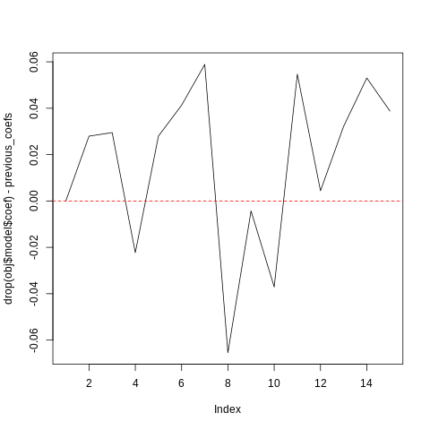
print(summary(previous_coefs))
print(summary(drop(obj$model$coef) - previous_coefs))
plot(drop(obj$model$coef) - previous_coefs, type='l')
abline(h = 0, lty=2, col="red")
Elapsed:  0.003 s
    Min.  1st Qu.   Median     Mean  3rd Qu.     Max.
-0.96778 -0.51401 -0.16335 -0.05234  0.31900  0.98482
     Min.   1st Qu.    Median      Mean   3rd Qu.      Max.
-0.065436 -0.002152  0.027994  0.015974  0.040033  0.058892
%%R

print(obj$summary(new_X_test, y=new_y_test, show_progress=FALSE))
$R_squared
[1] 0.6692541

$R_squared_adj
[1] -2.638205

$Residuals
   Min. 1st Qu.  Median    Mean 3rd Qu.    Max.
-4.5014 -2.2111 -0.5532 -0.3928  1.3495  3.9206

$Coverage_rate
[1] 100

$citests
         estimate        lower        upper      p-value signif
cyl   -41.4815528  -43.6039915  -39.3591140 1.306085e-13    ***
disp   -0.5937584   -0.7014857   -0.4860311 1.040246e-07    ***
hp     -1.0226867   -1.2175471   -0.8278263 1.719172e-07    ***
drat   84.5859637   73.2987057   95.8732217 4.178658e-09    ***
wt   -169.1047879 -189.5595154 -148.6500603 1.469605e-09    ***
qsec   22.3026258   15.1341951   29.4710566 2.772362e-05    ***
vs    113.3209911   88.3101728  138.3318093 7.599984e-07    ***
am    175.1639102  139.5755741  210.7522464 3.304560e-07    ***
gear   44.3270639   36.1456398   52.5084881 1.240722e-07    ***
carb  -59.6511203  -69.8576126  -49.4446280 5.677270e-08    ***

$effects
── Data Summary ────────────────────────
                           Values
Name                       effects
Number of rows             12
Number of columns          10
_______________________
Column type frequency:
  numeric                  10
________________________
Group variables            None

── Variable type: numeric ──────────────────────────────────────────────────────
   skim_variable     mean     sd       p0      p25      p50      p75     p100
 1 cyl            -41.5    3.34   -43.4    -43.4    -43.3    -41.7    -34.5
 2 disp            -0.594  0.170   -0.916   -0.635   -0.505   -0.505   -0.356
 3 hp              -1.02   0.307   -1.44    -1.40    -0.877   -0.768   -0.768
 4 drat            84.6   17.8     59.5     76.7     89.5     89.5    128.
 5 wt            -169.    32.2   -204.    -199.    -166.    -138.    -138.
 6 qsec            22.3   11.3     13.3     13.3     17.4     29.2     40.1
 7 vs             113.    39.4     59.6     94.4     94.4    117.     191.
 8 am             175.    56.0    124.     124.     153.     226.     245.
 9 gear            44.3   12.9     26.3     38.7     47.9     47.9     76.0
10 carb           -59.7   16.1    -77.3    -74.6    -58.2    -44.4    -44.4
   hist
 1 ▇▁▁▁▂
 2 ▂▁▃▇▁
 3 ▅▁▁▂▇
 4 ▂▃▇▁▁
 5 ▇▁▁▁▇
 6 ▇▂▁▁▃
 7 ▁▇▃▁▂
 8 ▇▁▁▂▃
 9 ▂▃▇▁▁
10 ▇▁▁▁▇
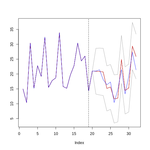
%%R

res <- obj$predict(X = new_X_test)

new_y_train <- c(y_train, newy)

plot(c(new_y_train, res$preds), type='l',
    main="",
    ylab="",
    ylim = c(min(c(res$upper, res$lower, y)),
             max(c(res$upper, res$lower, y))))
lines(c(new_y_train, res$upper), col="gray60")
lines(c(new_y_train, res$lower), col="gray60")
lines(c(new_y_train, res$preds), col = "red")
lines(c(new_y_train, new_y_test), col = "blue")
abline(v = length(y_train), lty=2, col="black")
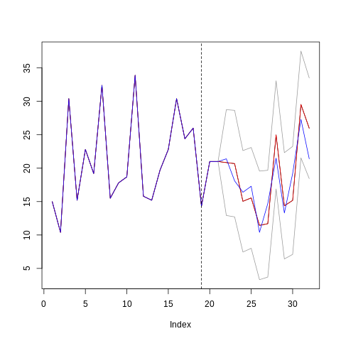
%%R

newx <- X_test[2, ]
newy <- y_test[2]

new_X_test <- X_test[-c(1, 2), ]
new_y_test <- y_test[-c(1, 2)]

t0 <- proc.time()[3]
obj$update(newx, newy, method = "polyak", alpha = 0.9)
cat("Elapsed: ", proc.time()[3] - t0, "s \n")

print(obj$summary(new_X_test, y=new_y_test, show_progress=FALSE))


res <- obj$predict(X = new_X_test)

new_y_train <- c(y_train, y_test[c(1, 2)])

plot(c(new_y_train, res$preds), type='l',
    main="",
    ylab="",
    ylim = c(min(c(res$upper, res$lower, y)),
             max(c(res$upper, res$lower, y))))
lines(c(new_y_train, res$upper), col="gray60")
lines(c(new_y_train, res$lower), col="gray60")
lines(c(new_y_train, res$preds), col = "red")
lines(c(new_y_train, new_y_test), col = "blue")
abline(v = length(y_train), lty=2, col="black")
Elapsed:  0.003 s
$R_squared
[1] 0.6426871

$R_squared_adj
[1] -Inf

$Residuals
   Min. 1st Qu.  Median    Mean 3rd Qu.    Max.
-4.5686 -2.4084 -1.0397 -0.3897  1.5507  4.0215

$Coverage_rate
[1] 100

$citests
         estimate        lower        upper      p-value signif
cyl   -42.1261096  -44.5327541  -39.7194651 2.932516e-12    ***
disp   -0.6256505   -0.7347381   -0.5165629 1.613495e-07    ***
hp     -1.0139634   -1.2198651   -0.8080617 6.747693e-07    ***
drat   82.8645391   74.8033348   90.9257434 5.680663e-10    ***
wt   -170.7891742 -193.1932631 -148.3850853 1.053193e-08    ***
qsec   22.2365552   13.9564091   30.5167012 1.350094e-04    ***
vs    119.1784891   94.0163626  144.3406157 9.681321e-07    ***
am    174.2138307  134.1390652  214.2885963 2.127371e-06    ***
gear   42.7943293   36.9622907   48.6263678 1.523695e-08    ***
carb  -59.4034661  -70.5135723  -48.2933599 3.127231e-07    ***

$effects
── Data Summary ────────────────────────
                           Values
Name                       effects
Number of rows             11
Number of columns          10
_______________________
Column type frequency:
  numeric                  10
________________________
Group variables            None

── Variable type: numeric ──────────────────────────────────────────────────────
   skim_variable     mean     sd       p0      p25      p50      p75     p100
 1 cyl            -42.1    3.58   -44.1    -44.1    -44.1    -43.0    -34.9
 2 disp            -0.626  0.162   -0.933   -0.643   -0.514   -0.514   -0.514
 3 hp              -1.01   0.306   -1.47    -1.24    -0.787   -0.787   -0.787
 4 drat            82.9   12.0     61.2     79.6     91.7     91.7     91.7
 5 wt            -171.    33.3   -210.    -204.    -142.    -142.    -142.
 6 qsec            22.2   12.3     13.2     13.2     13.2     30.7     41.2
 7 vs             119.    37.5     96.0     96.0     96.0    117.     193.
 8 am             174.    59.7    123.     123.     123.     233.     247.
 9 gear            42.8    8.68    27.1     40.4     49.2     49.2     49.2
10 carb           -59.4   16.5    -78.8    -76.0    -45.1    -45.1    -45.1
   hist
 1 ▇▁▁▁▂
 2 ▂▁▁▃▇
 3 ▃▁▁▂▇
 4 ▂▁▁▃▇
 5 ▇▁▁▁▇
 6 ▇▂▁▁▃
 7 ▇▃▁▁▂
 8 ▇▁▁▂▃
 9 ▂▁▁▃▇
10 ▇▁▁▁▇
2 - Python version
!pip install git+https://github.com/Techtonique/learningmachine_python.git --verbose
import pandas as pd
import numpy as np
import warnings
import learningmachine as lm


# Load the mtcars dataset
data = pd.read_csv("https://raw.githubusercontent.com/plotly/datasets/master/mtcars.csv")
X = data.drop("mpg", axis=1).values
X = pd.DataFrame(X).iloc[:,1:]
X = X.astype(np.float16)
X.columns = ["cyl","disp","hp","drat","wt","qsec","vs","am","gear","carb"]
y = data["mpg"].values
display(X.describe())
display(X.head())
display(X.dtypes)
| cyl | disp | hp | drat | wt | qsec | vs | am | gear | carb | |
|---|---|---|---|---|---|---|---|---|---|---|
| count | 32.000000 | 32.000000 | 32.0000 | 32.000000 | 32.000000 | 32.000000 | 32.000000 | 32.000000 | 32.000000 | 32.000000 |
| mean | 6.187500 | 230.750000 | 146.7500 | 3.595703 | 3.216797 | 17.843750 | 0.437500 | 0.406250 | 3.687500 | 2.812500 |
| std | 1.786133 | 123.937500 | 68.5625 | 0.534668 | 0.978516 | 1.788086 | 0.503906 | 0.499023 | 0.737793 | 1.615234 |
| min | 4.000000 | 71.125000 | 52.0000 | 2.759766 | 1.512695 | 14.500000 | 0.000000 | 0.000000 | 3.000000 | 1.000000 |
| 25% | 4.000000 | 120.828125 | 96.5000 | 3.080078 | 2.580566 | 16.898438 | 0.000000 | 0.000000 | 3.000000 | 2.000000 |
| 50% | 6.000000 | 196.312500 | 123.0000 | 3.694336 | 3.325195 | 17.703125 | 0.000000 | 0.000000 | 4.000000 | 2.000000 |
| 75% | 8.000000 | 326.000000 | 180.0000 | 3.919922 | 3.610352 | 18.906250 | 1.000000 | 1.000000 | 4.000000 | 4.000000 |
| max | 8.000000 | 472.000000 | 335.0000 | 4.929688 | 5.425781 | 22.906250 | 1.000000 | 1.000000 | 5.000000 | 8.000000 |
| cyl | disp | hp | drat | wt | qsec | vs | am | gear | carb | |
|---|---|---|---|---|---|---|---|---|---|---|
| 0 | 6.0 | 160.0 | 110.0 | 3.900391 | 2.619141 | 16.453125 | 0.0 | 1.0 | 4.0 | 4.0 |
| 1 | 6.0 | 160.0 | 110.0 | 3.900391 | 2.875000 | 17.015625 | 0.0 | 1.0 | 4.0 | 4.0 |
| 2 | 4.0 | 108.0 | 93.0 | 3.849609 | 2.320312 | 18.609375 | 1.0 | 1.0 | 4.0 | 1.0 |
| 3 | 6.0 | 258.0 | 110.0 | 3.080078 | 3.214844 | 19.437500 | 1.0 | 0.0 | 3.0 | 1.0 |
| 4 | 8.0 | 360.0 | 175.0 | 3.150391 | 3.439453 | 17.015625 | 0.0 | 0.0 | 3.0 | 2.0 |
| 0 | |
|---|---|
| cyl | float16 |
| disp | float16 |
| hp | float16 |
| drat | float16 |
| wt | float16 |
| qsec | float16 |
| vs | float16 |
| am | float16 |
| gear | float16 |
| carb | float16 |
y.dtype
dtype('float64')
X
| cyl | disp | hp | drat | wt | qsec | vs | am | gear | carb | |
|---|---|---|---|---|---|---|---|---|---|---|
| 0 | 6.0 | 160.0000 | 110.0 | 3.900391 | 2.619141 | 16.453125 | 0.0 | 1.0 | 4.0 | 4.0 |
| 1 | 6.0 | 160.0000 | 110.0 | 3.900391 | 2.875000 | 17.015625 | 0.0 | 1.0 | 4.0 | 4.0 |
| 2 | 4.0 | 108.0000 | 93.0 | 3.849609 | 2.320312 | 18.609375 | 1.0 | 1.0 | 4.0 | 1.0 |
| 3 | 6.0 | 258.0000 | 110.0 | 3.080078 | 3.214844 | 19.437500 | 1.0 | 0.0 | 3.0 | 1.0 |
| 4 | 8.0 | 360.0000 | 175.0 | 3.150391 | 3.439453 | 17.015625 | 0.0 | 0.0 | 3.0 | 2.0 |
| 5 | 6.0 | 225.0000 | 105.0 | 2.759766 | 3.460938 | 20.218750 | 1.0 | 0.0 | 3.0 | 1.0 |
| 6 | 8.0 | 360.0000 | 245.0 | 3.210938 | 3.570312 | 15.843750 | 0.0 | 0.0 | 3.0 | 4.0 |
| 7 | 4.0 | 146.7500 | 62.0 | 3.689453 | 3.189453 | 20.000000 | 1.0 | 0.0 | 4.0 | 2.0 |
| 8 | 4.0 | 140.7500 | 95.0 | 3.919922 | 3.150391 | 22.906250 | 1.0 | 0.0 | 4.0 | 2.0 |
| 9 | 6.0 | 167.6250 | 123.0 | 3.919922 | 3.439453 | 18.296875 | 1.0 | 0.0 | 4.0 | 4.0 |
| 10 | 6.0 | 167.6250 | 123.0 | 3.919922 | 3.439453 | 18.906250 | 1.0 | 0.0 | 4.0 | 4.0 |
| 11 | 8.0 | 275.7500 | 180.0 | 3.070312 | 4.070312 | 17.406250 | 0.0 | 0.0 | 3.0 | 3.0 |
| 12 | 8.0 | 275.7500 | 180.0 | 3.070312 | 3.730469 | 17.593750 | 0.0 | 0.0 | 3.0 | 3.0 |
| 13 | 8.0 | 275.7500 | 180.0 | 3.070312 | 3.779297 | 18.000000 | 0.0 | 0.0 | 3.0 | 3.0 |
| 14 | 8.0 | 472.0000 | 205.0 | 2.929688 | 5.250000 | 17.984375 | 0.0 | 0.0 | 3.0 | 4.0 |
| 15 | 8.0 | 460.0000 | 215.0 | 3.000000 | 5.425781 | 17.812500 | 0.0 | 0.0 | 3.0 | 4.0 |
| 16 | 8.0 | 440.0000 | 230.0 | 3.230469 | 5.343750 | 17.421875 | 0.0 | 0.0 | 3.0 | 4.0 |
| 17 | 4.0 | 78.6875 | 66.0 | 4.078125 | 2.199219 | 19.468750 | 1.0 | 1.0 | 4.0 | 1.0 |
| 18 | 4.0 | 75.6875 | 52.0 | 4.929688 | 1.615234 | 18.515625 | 1.0 | 1.0 | 4.0 | 2.0 |
| 19 | 4.0 | 71.1250 | 65.0 | 4.218750 | 1.834961 | 19.906250 | 1.0 | 1.0 | 4.0 | 1.0 |
| 20 | 4.0 | 120.1250 | 97.0 | 3.699219 | 2.464844 | 20.015625 | 1.0 | 0.0 | 3.0 | 1.0 |
| 21 | 8.0 | 318.0000 | 150.0 | 2.759766 | 3.519531 | 16.875000 | 0.0 | 0.0 | 3.0 | 2.0 |
| 22 | 8.0 | 304.0000 | 150.0 | 3.150391 | 3.435547 | 17.296875 | 0.0 | 0.0 | 3.0 | 2.0 |
| 23 | 8.0 | 350.0000 | 245.0 | 3.730469 | 3.839844 | 15.406250 | 0.0 | 0.0 | 3.0 | 4.0 |
| 24 | 8.0 | 400.0000 | 175.0 | 3.080078 | 3.845703 | 17.046875 | 0.0 | 0.0 | 3.0 | 2.0 |
| 25 | 4.0 | 79.0000 | 66.0 | 4.078125 | 1.934570 | 18.906250 | 1.0 | 1.0 | 4.0 | 1.0 |
| 26 | 4.0 | 120.3125 | 91.0 | 4.429688 | 2.140625 | 16.703125 | 0.0 | 1.0 | 5.0 | 2.0 |
| 27 | 4.0 | 95.1250 | 113.0 | 3.769531 | 1.512695 | 16.906250 | 1.0 | 1.0 | 5.0 | 2.0 |
| 28 | 8.0 | 351.0000 | 264.0 | 4.218750 | 3.169922 | 14.500000 | 0.0 | 1.0 | 5.0 | 4.0 |
| 29 | 6.0 | 145.0000 | 175.0 | 3.619141 | 2.769531 | 15.500000 | 0.0 | 1.0 | 5.0 | 6.0 |
| 30 | 8.0 | 301.0000 | 335.0 | 3.539062 | 3.570312 | 14.601562 | 0.0 | 1.0 | 5.0 | 8.0 |
| 31 | 4.0 | 121.0000 | 109.0 | 4.109375 | 2.779297 | 18.593750 | 1.0 | 1.0 | 4.0 | 2.0 |
# Split the data into training and testing sets
from sklearn.model_selection import train_test_split
X_train, X_test, y_train, y_test = train_test_split(X, y, test_size=0.2, random_state=123)

# Create a Bayesian RVFL regressor object
obj = lm.Regressor(method = "bayesianrvfl", nb_hidden = 5)

# Fit the model using the training data
obj.fit(X_train, y_train, reg_lambda=12.9155)

# Print the summary of the model
print(obj.summary(X_test, y=y_test, show_progress=False))
$R_squared
[1] 0.6416309

$R_squared_adj
[1] 1.537554

$Residuals
   Min. 1st Qu.  Median    Mean 3rd Qu.    Max.
-4.0724 -2.0122 -0.1018 -0.1941  1.4361  3.9676

$Coverage_rate
[1] 100

$citests
         estimate       lower        upper      p-value signif
cyl   -24.5943583  -40.407994   -8.7807230 8.909365e-03     **
disp   -0.2419797   -0.370835   -0.1131245 3.711077e-03     **
hp     -1.5734483   -1.722903   -1.4239939 2.255640e-07    ***
drat  142.5646192  124.575179  160.5540599 1.217808e-06    ***
wt   -144.8871352 -158.911143 -130.8631275 2.523441e-07    ***
qsec   46.8290859   27.829411   65.8287611 9.388045e-04    ***
vs     75.0555146   30.645127  119.4659017 6.110043e-03     **
am    207.5935234  133.205572  281.9814744 4.843095e-04    ***
gear   73.6892658   60.186232   87.1922995 1.091470e-05    ***
carb  -71.2974988  -79.480400  -63.1145974 6.944475e-07    ***

$effects
── Data Summary ────────────────────────
                           Values
Name                       effects
Number of rows             7
Number of columns          10
_______________________
Column type frequency:
  numeric                  10
________________________
Group variables            None

── Variable type: numeric ──────────────────────────────────────────────────────
   skim_variable     mean     sd       p0      p25      p50      p75       p100
 1 cyl            -24.6   17.1    -38.5    -38.5    -33.4    -12.4      1.66
 2 disp            -0.242  0.139   -0.351   -0.351   -0.285   -0.181    0.00546
 3 hp              -1.57   0.162   -1.90    -1.61    -1.48    -1.47    -1.47
 4 drat           143.    19.5    125.     125.     141.     154.     174.
 5 wt            -145.    15.2   -167.    -152.    -142.    -142.    -117.
 6 qsec            46.8   20.5     14.1     35.3     55.7     62.4     62.4
 7 vs              75.1   48.0     37.2     37.2     58.7     93.9    167.
 8 am             208.    80.4     64.3    168.     250.     267.     267.
 9 gear            73.7   14.6     60.6     60.6     72.7     82.1     96.9
10 carb           -71.3    8.85   -84.4    -75.2    -69.7    -69.7    -55.2
   hist
 1 ▇▁▂▁▃
 2 ▇▂▁▂▂
 3 ▂▁▁▃▇
 4 ▇▂▂▂▂
 5 ▂▅▇▁▂
 6 ▃▁▁▂▇
 7 ▇▁▃▁▂
 8 ▂▂▁▂▇
 9 ▇▂▂▂▂
10 ▂▅▇▁▂
# Select the first test sample
newx = X_test.iloc[0,:]
newy = y_test[0]

# Update the model with the new sample
new_X_test = X_test[1:]
new_y_test = y_test[1:]
obj.update(newx, newy, method="polyak", alpha=0.9)

# Print the summary of the model
print(obj.summary(new_X_test, y=new_y_test, show_progress=False))
$R_squared
[1] 0.6051442

$R_squared_adj
[1] 1.394856

$Residuals
   Min. 1st Qu.  Median    Mean 3rd Qu.    Max.
-4.6214 -2.5055 -1.5003 -0.8308  1.2738  3.2794

$Coverage_rate
[1] 100

$citests
         estimate        lower       upper      p-value signif
cyl   -30.0502823  -48.4171958  -11.683369 8.442658e-03     **
disp   -0.2958477   -0.4386085   -0.153087 3.121989e-03     **
hp     -1.6053302   -1.6789750   -1.531685 3.424156e-08    ***
drat  153.7968829  131.5239191  176.069847 1.041460e-05    ***
wt   -155.1954135 -174.4144275 -135.976399 4.804729e-06    ***
qsec   49.8967685   26.9993778   72.794159 2.504905e-03     **
vs     87.4170764   32.4599776  142.374175 9.457226e-03     **
am    214.5918910  119.8712855  309.312496 2.108825e-03     **
gear   83.1355825   65.3159018  100.955263 7.110354e-05    ***
carb  -77.1384645  -88.2087477  -66.068181 9.958425e-06    ***

$effects
── Data Summary ────────────────────────
                           Values
Name                       effects
Number of rows             6
Number of columns          10
_______________________
Column type frequency:
  numeric                  10
________________________
Group variables            None

── Variable type: numeric ──────────────────────────────────────────────────────
   skim_variable     mean      sd       p0      p25      p50      p75      p100
 1 cyl            -30.1   17.5     -42.5    -42.5    -39.9    -17.7     -4.35
 2 disp            -0.296  0.136    -0.377   -0.377   -0.343   -0.308   -0.0269
 3 hp              -1.61   0.0702   -1.70    -1.66    -1.57    -1.57    -1.53
 4 drat           154.    21.2     137.     137.     144.     169.     185.
 5 wt            -155.    18.3    -182.    -160.    -154.    -154.    -125.
 6 qsec            49.9   21.8      18.8     33.3     60.6     66.6     66.6
 7 vs              87.4   52.4      46.7     46.7     73.7    105.     178.
 8 am             215.    90.3      65.6    169.     266.     275.     275.
 9 gear            83.1   17.0      70.0     70.0     75.5     94.1    109.
10 carb           -77.1   10.5     -92.5    -79.9    -76.6    -76.6    -59.7
   hist
 1 ▇▁▁▁▃
 2 ▇▂▁▁▂
 3 ▅▁▁▇▂
 4 ▇▂▁▁▅
 5 ▂▂▇▁▂
 6 ▅▁▁▂▇
 7 ▇▁▅▁▂
 8 ▂▂▁▁▇
 9 ▇▂▁▂▂
10 ▂▂▇▁▂
Citation
For attribution, please cite this work as:
T. Moudiki (2024-09-10). Adaptive (online/streaming) learning with uncertainty quantification using Polyak averaging in learningmachine. Retrieved from https://thierrymoudiki.github.io/blog/2024/09/10/python/r/adaptive-polyak
BibTeX citation (remove empty spaces)
        @misc{ tmoudiki20240910,
          author = { T. Moudiki },
          title = { Adaptive (online/streaming) learning with uncertainty quantification using Polyak averaging in learningmachine },
          url = { https://thierrymoudiki.github.io/blog/2024/09/10/python/r/adaptive-polyak },
          year = { 2024 } }

Previous publications
- Fast conformal prediction (no refitting) for some Machine Learning models via closed-form jackknife plus Jun 27, 2026
- Using scikit-learn models in R easily with the tisthemachinelearner package Jun 21, 2026
- No-Code Machine Learning in Excel with the Techtonique API Jun 14, 2026
- How Conformal Prediction Makes Linear Models Good Enough — An Example Using R Package mlS3 Jun 7, 2026
- Techtonique dot net, the Machine Learning web API, is back online (but more like a passion project for now) May 31, 2026
- Conformalized TabICL: Prediction Intervals for a State-Of-The-Art Tabular Foundation Model in Python and R May 21, 2026
- Conformalized TabPFN: Prediction Intervals for a Pretrained Transformer for Tabular Data in Python and R May 17, 2026
- Probabilistic Time Series Cross-Validation with R package crossvalidation May 16, 2026
- One interface, (Almost) Every Classifier (and Regressor): unifiedml v0.3.0 May 9, 2026
- You Don't Need to Learn All the Weights on tabular data: The Case for rvflnet (a nonlinear expressive glmnet) on regression, classification and survival analysis May 2, 2026
- Survival analysis with sklearn, glmnet, keras, pytorch, lightgbm, xgboost, nnetsauce, mlsauce Part 2 Apr 28, 2026
- Any Sklearn Regressor as a Survival Model — Does It Actually Work? Benchmarking vs Established Packages Apr 26, 2026
- Conformal Optimization Beats Bayesian Optimization, Optuna and Random Search on 72 classification Datasets Apr 19, 2026
- `mlS3` — A Unified S3 Machine Learning Interface in R Apr 12, 2026
- One interface, (Almost) Every Classifier: unifiedml v0.2.1 Apr 4, 2026
- Techtonique dot net is down until further notice Apr 1, 2026
- Explaining Time-Series Forecasts with Sensitivity Analysis (ahead::dynrmf and external regressors) Mar 29, 2026
- Python version of 'Option pricing using time series models as market price of risk Pt.3' Mar 22, 2026
- Option pricing using time series models as market price of risk Pt.3 Mar 16, 2026
- Explaining Time-Series Forecasts with Exact Shapley Values (ahead::dynrmf with external regressors applied to scenarios) Mar 8, 2026
- My Presentation at Risk 2026: Lightweight Transfer Learning for Financial Forecasting Mar 1, 2026
- nnetsauce with and without jax for GPU acceleration Feb 23, 2026
- Understanding Boosted Configuration Networks (combined neural networks and boosting): An Intuitive Guide Through Their Hyperparameters Feb 16, 2026
- R version of Python package survivalist, for model-agnostic survival analysis Feb 9, 2026
- Presenting Lightweight Transfer Learning for Financial Forecasting (Risk 2026) Feb 4, 2026
- Option pricing using time series models as market price of risk Feb 1, 2026
- Enhancing Time Series Forecasting (ahead::ridge2f) with Attention-Based Context Vectors (ahead::contextridge2f) Jan 31, 2026
- Overfitting and scaling (on GPU T4) tests on nnetsauce.CustomRegressor Jan 29, 2026
- Beyond Cross-validation: Hyperparameter Optimization via Generalization Gap Modeling Jan 25, 2026
- GPopt for Machine Learning (hyperparameters' tuning) Jan 21, 2026
- rtopy: an R to Python bridge -- novelties Jan 8, 2026
- Python examples for 'Beyond Nelson-Siegel and splines: A model- agnostic Machine Learning framework for discount curve calibration, interpolation and extrapolation' Jan 3, 2026
- Forecasting benchmark: Dynrmf (a new serious competitor in town) vs Theta Method on M-Competitions and Tourism competitition Jan 1, 2026
- Finally figured out a way to port python packages to R using uv and reticulate: example with nnetsauce Dec 17, 2025
- Overfitting Random Fourier Features: Universal Approximation Property Dec 13, 2025
- Counterfactual Scenario Analysis with ahead::ridge2f Dec 11, 2025
- Zero-Shot Probabilistic Time Series Forecasting with TabPFN 2.5 and nnetsauce Dec 10, 2025
- ARIMA Pricing: Semi-Parametric Market price of risk for Risk-Neutral Pricing (code + preprint) Dec 7, 2025
- Analyzing Paper Reviews with LLMs: I Used ChatGPT, DeepSeek, Qwen, Mistral, Gemini, and Claude (and you should too + publish the analysis) Dec 3, 2025
- tisthemachinelearner: New Workflow with uv for R Integration of scikit-learn Dec 1, 2025
- (ICYMI) RPweave: Unified R + Python + LaTeX System using uv Nov 21, 2025
- unifiedml: A Unified Machine Learning Interface for R, is now on CRAN + Discussion about AI replacing humans Nov 16, 2025
- Context-aware Theta forecasting Method: Extending Classical Time Series Forecasting with Machine Learning Nov 13, 2025
- unifiedml in R: A Unified Machine Learning Interface Nov 5, 2025
- Deterministic Shift Adjustment in Arbitrage-Free Pricing (historical to risk-neutral short rates) Oct 28, 2025
- New instantaneous short rates models with their deterministic shift adjustment, for historical and risk-neutral simulation Oct 27, 2025
- RPweave: Unified R + Python + LaTeX System using uv Oct 19, 2025
- GAN-like Synthetic Data Generation Examples (on univariate, multivariate distributions, digits recognition, Fashion-MNIST, stock returns, and Olivetti faces) with DistroSimulator Oct 19, 2025
- R port of llama2.c Oct 9, 2025
- Native uncertainty quantification for time series with NGBoost Oct 8, 2025
- NGBoost (Natural Gradient Boosting) for Regression, Classification, Time Series forecasting and Reserving Oct 6, 2025
- Real-time pricing with a pretrained probabilistic stock return model Oct 1, 2025
- Combining any model with GARCH(1,1) for probabilistic stock forecasting Sep 23, 2025
- Generating Synthetic Data with R-vine Copulas using esgtoolkit in R Sep 21, 2025
- Reimagining Equity Solvency Capital Requirement Approximation (one of my Master's Thesis subjects): From Bilinear Interpolation to Probabilistic Machine Learning Sep 16, 2025
- Transfer Learning using ahead::ridge2f on synthetic stocks returns Pt.2: synthetic data generation Sep 9, 2025
- Transfer Learning using ahead::ridge2f on synthetic stocks returns Sep 8, 2025
- I'm supposed to present 'Conformal Predictive Simulations for Univariate Time Series' at COPA CONFERENCE 2025 in London... Sep 4, 2025
- external regressors in ahead::dynrmf's interface for Machine learning forecasting Sep 1, 2025
- Another interesting decision, now for 'Beyond Nelson-Siegel and splines: A model-agnostic Machine Learning framework for discount curve calibration, interpolation and extrapolation' Aug 20, 2025
- Boosting any randomized based learner for regression, classification and univariate/multivariate time series forcasting Jul 26, 2025
- New nnetsauce version with CustomBackPropRegressor (CustomRegressor with Backpropagation) and ElasticNet2Regressor (Ridge2 with ElasticNet regularization) Jul 15, 2025
- mlsauce (home to a model-agnostic gradient boosting algorithm) can now be installed from PyPI. Jul 10, 2025
- A user-friendly graphical interface to techtonique dot net's API (will eventually contain graphics). Jul 8, 2025
- Calling =TECHTO_MLCLASSIFICATION for Machine Learning supervised CLASSIFICATION in Excel is just a matter of copying and pasting Jul 7, 2025
- Calling =TECHTO_MLREGRESSION for Machine Learning supervised regression in Excel is just a matter of copying and pasting Jul 6, 2025
- Calling =TECHTO_RESERVING and =TECHTO_MLRESERVING for claims triangle reserving in Excel is just a matter of copying and pasting Jul 5, 2025
- Calling =TECHTO_SURVIVAL for Survival Analysis in Excel is just a matter of copying and pasting Jul 4, 2025
- Calling =TECHTO_SIMULATION for Stochastic Simulation in Excel is just a matter of copying and pasting Jul 3, 2025
- Calling =TECHTO_FORECAST for forecasting in Excel is just a matter of copying and pasting Jul 2, 2025
- Random Vector Functional Link (RVFL) artificial neural network with 2 regularization parameters successfully used for forecasting/synthetic simulation in professional settings: Extensions (including Bayesian) Jul 1, 2025
- R version of 'Backpropagating quasi-randomized neural networks' Jun 24, 2025
- Backpropagating quasi-randomized neural networks Jun 23, 2025
- Beyond ARMA-GARCH: leveraging any statistical model for volatility forecasting Jun 21, 2025
- Stacked generalization (Machine Learning model stacking) + conformal prediction for forecasting with ahead::mlf Jun 18, 2025
- An Overfitting dilemma: XGBoost Default Hyperparameters vs GenericBooster + LinearRegression Default Hyperparameters Jun 14, 2025
- Programming language-agnostic reserving using RidgeCV, LightGBM, XGBoost, and ExtraTrees Machine Learning models Jun 13, 2025
- Free R, Python and SQL editors in techtonique dot net Jun 9, 2025
- Beyond Nelson-Siegel and splines: A model-agnostic Machine Learning framework for discount curve calibration, interpolation and extrapolation Jun 7, 2025
- scikit-learn, glmnet, xgboost, lightgbm, pytorch, keras, nnetsauce in probabilistic Machine Learning (for longitudinal data) Reserving (work in progress) Jun 6, 2025
- R version of Probabilistic Machine Learning (for longitudinal data) Reserving (work in progress) Jun 5, 2025
- Probabilistic Machine Learning (for longitudinal data) Reserving (work in progress) Jun 4, 2025
- Python version of Beyond ARMA-GARCH: leveraging model-agnostic Quasi-Randomized networks and conformal prediction for nonparametric probabilistic stock forecasting (ML-ARCH) Jun 3, 2025
- Beyond ARMA-GARCH: leveraging model-agnostic Machine Learning and conformal prediction for nonparametric probabilistic stock forecasting (ML-ARCH) Jun 2, 2025
- Permutations and SHAPley values for feature importance in techtonique dot net's API (with R + Python + the command line) Jun 1, 2025
- Which patient is going to survive longer? Another guide to using techtonique dot net's API (with R + Python + the command line) for survival analysis May 31, 2025
- A Guide to Using techtonique.net's API and rush for simulating and plotting Stochastic Scenarios May 30, 2025
- Simulating Stochastic Scenarios with Diffusion Models: A Guide to Using techtonique.net's API for the purpose May 29, 2025
- Will my apartment in 5th avenue be overpriced or not? Harnessing the power of www.techtonique.net (+ xgboost, lightgbm, catboost) to find out May 28, 2025
- How long must I wait until something happens: A Comprehensive Guide to Survival Analysis via an API May 27, 2025
- Harnessing the Power of techtonique.net: A Comprehensive Guide to Machine Learning Classification via an API May 26, 2025
- Quantile regression with any regressor -- Examples with RandomForestRegressor, RidgeCV, KNeighborsRegressor May 20, 2025
- Survival stacking: survival analysis translated as supervised classification in R and Python May 5, 2025
- 'Bayesian' optimization of hyperparameters in a R machine learning model using the bayesianrvfl package Apr 25, 2025
- A lightweight interface to scikit-learn in R: Bayesian and Conformal prediction Apr 21, 2025
- A lightweight interface to scikit-learn in R Pt.2: probabilistic time series forecasting in conjunction with ahead::dynrmf Apr 20, 2025
- Extending the Theta forecasting method to GLMs, GAMs, GLMBOOST and attention: benchmarking on Tourism, M1, M3 and M4 competition data sets (28000 series) Apr 14, 2025
- Extending the Theta forecasting method to GLMs and attention Apr 8, 2025
- Nonlinear conformalized Generalized Linear Models (GLMs) with R package 'rvfl' (and other models) Mar 31, 2025
- Probabilistic Time Series Forecasting (predictive simulations) in Microsoft Excel using Python, xlwings lite and www.techtonique.net Mar 28, 2025
- Conformalize (improved prediction intervals and simulations) any R Machine Learning model with misc::conformalize Mar 25, 2025
- My poster for the 18th FINANCIAL RISKS INTERNATIONAL FORUM by Institut Louis Bachelier/Fondation du Risque/Europlace Institute of Finance Mar 19, 2025
- Interpretable probabilistic kernel ridge regression using Matérn 3/2 kernels Mar 16, 2025
- (News from) Probabilistic Forecasting of univariate and multivariate Time Series using Quasi-Randomized Neural Networks (Ridge2) and Conformal Prediction Mar 9, 2025
- Word-Online: re-creating Karpathy's char-RNN (with supervised linear online learning of word embeddings) for text completion Mar 8, 2025
- CRAN-like repository for most recent releases of Techtonique's R packages Mar 2, 2025
- Presenting 'Online Probabilistic Estimation of Carbon Beta and Carbon Shapley Values for Financial and Climate Risk' at Institut Louis Bachelier Feb 27, 2025
- Web app with DeepSeek R1 and Hugging Face API for chatting Feb 23, 2025
- tisthemachinelearner: A Lightweight interface to scikit-learn with 2 classes, Classifier and Regressor (in Python and R) Feb 17, 2025
- R version of survivalist: Probabilistic model-agnostic survival analysis using scikit-learn, xgboost, lightgbm (and conformal prediction) Feb 12, 2025
- Model-agnostic global Survival Prediction of Patients with Myeloid Leukemia in QRT/Gustave Roussy Challenge (challengedata.ens.fr): Python's survivalist Quickstart Feb 10, 2025
- A simple test of the martingale hypothesis in esgtoolkit Feb 3, 2025
- Command Line Interface (CLI) for techtonique.net's API Jan 31, 2025
- Gradient-Boosting and Boostrap aggregating anything (alert: high performance): Part5, easier install and Rust backend Jan 27, 2025
- Just got a paper on conformal prediction REJECTED by International Journal of Forecasting despite evidence on 30,000 time series (and more). What's going on? Part2: 1311 time series from the Tourism competition Jan 20, 2025
- Techtonique is released! (with a tutorial in various programming languages and formats) Jan 14, 2025
- Univariate and Multivariate Probabilistic Forecasting with nnetsauce and TabPFN Jan 14, 2025
- Just got a paper on conformal prediction REJECTED by International Journal of Forecasting despite evidence on 30,000 time series (and more). What's going on? Jan 5, 2025
- Python and Interactive dashboard version of Stock price forecasting with Deep Learning: throwing power at the problem (and why it won't make you rich) Dec 31, 2024
- Stock price forecasting with Deep Learning: throwing power at the problem (and why it won't make you rich) Dec 29, 2024
- No-code Machine Learning Cross-validation and Interpretability in techtonique.net Dec 23, 2024
- survivalist: Probabilistic model-agnostic survival analysis using scikit-learn, glmnet, xgboost, lightgbm, pytorch, keras, nnetsauce and mlsauce Dec 15, 2024
- Model-agnostic 'Bayesian' optimization (for hyperparameter tuning) using conformalized surrogates in GPopt Dec 9, 2024
- You can beat Forecasting LLMs (Large Language Models a.k.a foundation models) with nnetsauce.MTS Pt.2: Generic Gradient Boosting Dec 1, 2024
- You can beat Forecasting LLMs (Large Language Models a.k.a foundation models) with nnetsauce.MTS Nov 24, 2024
- Unified interface and conformal prediction (calibrated prediction intervals) for R package forecast (and 'affiliates') Nov 23, 2024
- GLMNet in Python: Generalized Linear Models Nov 18, 2024
- Gradient-Boosting anything (alert: high performance): Part4, Time series forecasting Nov 10, 2024
- Predictive scenarios simulation in R, Python and Excel using Techtonique API Nov 3, 2024
- Chat with your tabular data in www.techtonique.net Oct 30, 2024
- Gradient-Boosting anything (alert: high performance): Part3, Histogram-based boosting Oct 28, 2024
- R editor and SQL console (in addition to Python editors) in www.techtonique.net Oct 21, 2024
- R and Python consoles + JupyterLite in www.techtonique.net Oct 15, 2024
- Gradient-Boosting anything (alert: high performance): Part2, R version Oct 14, 2024
- Gradient-Boosting anything (alert: high performance) Oct 6, 2024
- Benchmarking 30 statistical/Machine Learning models on the VN1 Forecasting -- Accuracy challenge Oct 4, 2024
- Automated random variable distribution inference using Kullback-Leibler divergence and simulating best-fitting distribution Oct 2, 2024
- Forecasting in Excel using Techtonique's Machine Learning APIs under the hood Sep 30, 2024
- Techtonique web app for data-driven decisions using Mathematics, Statistics, Machine Learning, and Data Visualization Sep 25, 2024
- Parallel for loops (Map or Reduce) + New versions of nnetsauce and ahead Sep 16, 2024
- Adaptive (online/streaming) learning with uncertainty quantification using Polyak averaging in learningmachine Sep 10, 2024
- New versions of nnetsauce and ahead Sep 9, 2024
- Prediction sets and prediction intervals for conformalized Auto XGBoost, Auto LightGBM, Auto CatBoost, Auto GradientBoosting Sep 2, 2024
- Quick/automated R package development workflow (assuming you're using macOS or Linux) Part2 Aug 30, 2024
- R package development workflow (assuming you're using macOS or Linux) Aug 27, 2024
- A new method for deriving a nonparametric confidence interval for the mean Aug 26, 2024
- Conformalized adaptive (online/streaming) learning using learningmachine in Python and R Aug 19, 2024
- Bayesian (nonlinear) adaptive learning Aug 12, 2024
- Auto XGBoost, Auto LightGBM, Auto CatBoost, Auto GradientBoosting Aug 5, 2024
- Copulas for uncertainty quantification in time series forecasting Jul 28, 2024
- Forecasting uncertainty: sequential split conformal prediction + Block bootstrap (web app) Jul 22, 2024
- learningmachine for Python (new version) Jul 15, 2024
- learningmachine v2.0.0: Machine Learning with explanations and uncertainty quantification Jul 8, 2024
- My presentation at ISF 2024 conference (slides with nnetsauce probabilistic forecasting news) Jul 3, 2024
- 10 uncertainty quantification methods in nnetsauce forecasting Jul 1, 2024
- Forecasting with XGBoost embedded in Quasi-Randomized Neural Networks Jun 24, 2024
- Forecasting Monthly Airline Passenger Numbers with Quasi-Randomized Neural Networks Jun 17, 2024
- Automated hyperparameter tuning using any conformalized surrogate Jun 9, 2024
- Recognizing handwritten digits with Ridge2Classifier Jun 3, 2024
- Forecasting the Economy May 27, 2024
- A detailed introduction to Deep Quasi-Randomized 'neural' networks May 19, 2024
- Probability of receiving a loan; using learningmachine May 12, 2024
- mlsauce's `v0.18.2`: various examples and benchmarks with dimension reduction May 6, 2024
- mlsauce's `v0.17.0`: boosting with Elastic Net, polynomials and heterogeneity in explanatory variables Apr 29, 2024
- mlsauce's `v0.13.0`: taking into account inputs heterogeneity through clustering Apr 21, 2024
- mlsauce's `v0.12.0`: prediction intervals for LSBoostRegressor Apr 15, 2024
- Conformalized predictive simulations for univariate time series on more than 250 data sets Apr 7, 2024
- learningmachine v1.1.2: for Python Apr 1, 2024
- learningmachine v1.0.0: prediction intervals around the probability of the event 'a tumor being malignant' Mar 25, 2024
- Bayesian inference and conformal prediction (prediction intervals) in nnetsauce v0.18.1 Mar 18, 2024
- Multiple examples of Machine Learning forecasting with ahead Mar 11, 2024
- rtopy (v0.1.1): calling R functions in Python Mar 4, 2024
- ahead forecasting (v0.10.0): fast time series model calibration and Python plots Feb 26, 2024
- A plethora of datasets at your fingertips Part3: how many times do couples cheat on each other? Feb 19, 2024
- nnetsauce's introduction as of 2024-02-11 (new version 0.17.0) Feb 11, 2024
- Tuning Machine Learning models with GPopt's new version Part 2 Feb 5, 2024
- Tuning Machine Learning models with GPopt's new version Jan 29, 2024
- Subsampling continuous and discrete response variables Jan 22, 2024
- DeepMTS, a Deep Learning Model for Multivariate Time Series Jan 15, 2024
- A classifier that's very accurate (and deep) Pt.2: there are > 90 classifiers in nnetsauce Jan 8, 2024
- learningmachine: prediction intervals for conformalized Kernel ridge regression and Random Forest Jan 1, 2024
- A plethora of datasets at your fingertips Part2: how many times do couples cheat on each other? Descriptive analytics, interpretability and prediction intervals using conformal prediction Dec 25, 2023
- Diffusion models in Python with esgtoolkit (Part2) Dec 18, 2023
- Diffusion models in Python with esgtoolkit Dec 11, 2023
- Julia packaging at the command line Dec 4, 2023
- Quasi-randomized nnetworks in Julia, Python and R Nov 27, 2023
- A plethora of datasets at your fingertips Nov 20, 2023
- A classifier that's very accurate (and deep) Nov 12, 2023
- mlsauce version 0.8.10: Statistical/Machine Learning with Python and R Nov 5, 2023
- AutoML in nnetsauce (randomized and quasi-randomized nnetworks) Pt.2: multivariate time series forecasting Oct 29, 2023
- AutoML in nnetsauce (randomized and quasi-randomized nnetworks) Oct 22, 2023
- Version v0.14.0 of nnetsauce for R and Python Oct 16, 2023
- A diffusion model: G2++ Oct 9, 2023
- Diffusion models in ESGtoolkit + announcements Oct 2, 2023
- An infinity of time series forecasting models in nnetsauce (Part 2 with uncertainty quantification) Sep 25, 2023
- (News from) forecasting in Python with ahead (progress bars and plots) Sep 18, 2023
- Forecasting in Python with ahead Sep 11, 2023
- Risk-neutralize simulations Sep 4, 2023
- Comparing cross-validation results using crossval_ml and boxplots Aug 27, 2023
- Reminder Apr 30, 2023
- Did you ask ChatGPT about who you are? Apr 16, 2023
- A new version of nnetsauce (randomized and quasi-randomized 'neural' networks) Apr 2, 2023
- Simple interfaces to the forecasting API Nov 23, 2022
- A web application for forecasting in Python, R, Ruby, C#, JavaScript, PHP, Go, Rust, Java, MATLAB, etc. Nov 2, 2022
- Prediction intervals (not only) for Boosted Configuration Networks in Python Oct 5, 2022
- Boosted Configuration (neural) Networks Pt. 2 Sep 3, 2022
- Boosted Configuration (_neural_) Networks for classification Jul 21, 2022
- A Machine Learning workflow using Techtonique Jun 6, 2022
- Super Mario Bros © in the browser using PyScript May 8, 2022
- News from ESGtoolkit, ycinterextra, and nnetsauce Apr 4, 2022
- Explaining a Keras _neural_ network predictions with the-teller Mar 11, 2022
- New version of nnetsauce -- various quasi-randomized networks Feb 12, 2022
- A dashboard illustrating bivariate time series forecasting with `ahead` Jan 14, 2022
- Hundreds of Statistical/Machine Learning models for univariate time series, using ahead, ranger, xgboost, and caret Dec 20, 2021
- Forecasting with `ahead` (Python version) Dec 13, 2021
- Tuning and interpreting LSBoost Nov 15, 2021
- Time series cross-validation using `crossvalidation` (Part 2) Nov 7, 2021
- Fast and scalable forecasting with ahead::ridge2f Oct 31, 2021
- Automatic Forecasting with `ahead::dynrmf` and Ridge regression Oct 22, 2021
- Forecasting with `ahead` Oct 15, 2021
- Classification using linear regression Sep 26, 2021
- `crossvalidation` and random search for calibrating support vector machines Aug 6, 2021
- parallel grid search cross-validation using `crossvalidation` Jul 31, 2021
- `crossvalidation` on R-universe, plus a classification example Jul 23, 2021
- Documentation and source code for GPopt, a package for Bayesian optimization Jul 2, 2021
- Hyperparameters tuning with GPopt Jun 11, 2021
- A forecasting tool (API) with examples in curl, R, Python May 28, 2021
- Bayesian Optimization with GPopt Part 2 (save and resume) Apr 30, 2021
- Bayesian Optimization with GPopt Apr 16, 2021
- Compatibility of nnetsauce and mlsauce with scikit-learn Mar 26, 2021
- Explaining xgboost predictions with the teller Mar 12, 2021
- An infinity of time series models in nnetsauce Mar 6, 2021
- New activation functions in mlsauce's LSBoost Feb 12, 2021
- 2020 recap, Gradient Boosting, Generalized Linear Models, AdaOpt with nnetsauce and mlsauce Dec 29, 2020
- A deeper learning architecture in nnetsauce Dec 18, 2020
- Classify penguins with nnetsauce's MultitaskClassifier Dec 11, 2020
- Bayesian forecasting for uni/multivariate time series Dec 4, 2020
- Generalized nonlinear models in nnetsauce Nov 28, 2020
- Boosting nonlinear penalized least squares Nov 21, 2020
- Statistical/Machine Learning explainability using Kernel Ridge Regression surrogates Nov 6, 2020
- NEWS Oct 30, 2020
- A glimpse into my PhD journey Oct 23, 2020
- Submitting R package to CRAN Oct 16, 2020
- Simulation of dependent variables in ESGtoolkit Oct 9, 2020
- Forecasting lung disease progression Oct 2, 2020
- New nnetsauce Sep 25, 2020
- Technical documentation Sep 18, 2020
- A new version of nnetsauce, and a new Techtonique website Sep 11, 2020
- Back next week, and a few announcements Sep 4, 2020
- Explainable 'AI' using Gradient Boosted randomized networks Pt2 (the Lasso) Jul 31, 2020
- LSBoost: Explainable 'AI' using Gradient Boosted randomized networks (with examples in R and Python) Jul 24, 2020
- nnetsauce version 0.5.0, randomized neural networks on GPU Jul 17, 2020
- Maximizing your tip as a waiter (Part 2) Jul 10, 2020
- New version of mlsauce, with Gradient Boosted randomized networks and stump decision trees Jul 3, 2020
- Announcements Jun 26, 2020
- Parallel AdaOpt classification Jun 19, 2020
- Comments section and other news Jun 12, 2020
- Maximizing your tip as a waiter Jun 5, 2020
- AdaOpt classification on MNIST handwritten digits (without preprocessing) May 29, 2020
- AdaOpt (a probabilistic classifier based on a mix of multivariable optimization and nearest neighbors) for R May 22, 2020
- AdaOpt May 15, 2020
- Custom errors for cross-validation using crossval::crossval_ml May 8, 2020
- Documentation+Pypi for the `teller`, a model-agnostic tool for Machine Learning explainability May 1, 2020
- Encoding your categorical variables based on the response variable and correlations Apr 24, 2020
- Linear model, xgboost and randomForest cross-validation using crossval::crossval_ml Apr 17, 2020
- Grid search cross-validation using crossval Apr 10, 2020
- Documentation for the querier, a query language for Data Frames Apr 3, 2020
- Time series cross-validation using crossval Mar 27, 2020
- On model specification, identification, degrees of freedom and regularization Mar 20, 2020
- Import data into the querier (now on Pypi), a query language for Data Frames Mar 13, 2020
- R notebooks for nnetsauce Mar 6, 2020
- Version 0.4.0 of nnetsauce, with fruits and breast cancer classification Feb 28, 2020
- Create a specific feed in your Jekyll blog Feb 21, 2020
- Git/Github for contributing to package development Feb 14, 2020
- Feedback forms for contributing Feb 7, 2020
- nnetsauce for R Jan 31, 2020
- A new version of nnetsauce (v0.3.1) Jan 24, 2020
- ESGtoolkit, a tool for Monte Carlo simulation (v0.2.0) Jan 17, 2020
- Search bar, new year 2020 Jan 10, 2020
- 2019 Recap, the nnetsauce, the teller and the querier Dec 20, 2019
- Understanding model interactions with the `teller` Dec 13, 2019
- Using the `teller` on a classifier Dec 6, 2019
- Benchmarking the querier's verbs Nov 29, 2019
- Composing the querier's verbs for data wrangling Nov 22, 2019
- Comparing and explaining model predictions with the teller Nov 15, 2019
- Tests for the significance of marginal effects in the teller Nov 8, 2019
- Introducing the teller Nov 1, 2019
- Introducing the querier Oct 25, 2019
- Prediction intervals for nnetsauce models Oct 18, 2019
- Using R in Python for statistical learning/data science Oct 11, 2019
- Model calibration with `crossval` Oct 4, 2019
- Bagging in the nnetsauce Sep 25, 2019
- Adaboost learning with nnetsauce Sep 18, 2019
- Change in blog's presentation Sep 4, 2019
- nnetsauce on Pypi Jun 5, 2019
- More nnetsauce (examples of use) May 9, 2019
- nnetsauce Mar 13, 2019
- crossval Mar 13, 2019
- test Mar 10, 2019
Comments powered by Talkyard.