In this post, we will explore the use of generalization gap modeling for hyperparameter optimization of a LightGBM model. A surrogate model (here a kernel ridge regression model) is fitted on the gap between a model’s cross-validation error and test set error. Our surrogate model could then be used to predict the generalization gap for new hyperparameter combinations, and obtain various insights on the LightGBM model’s ability to generalize on unseen data.
More details can be found in this document https://www.researchgate.net/publication/398667338_Beyond_Performance_Hyperparameter_Optimization_via_Direct_Generalization_Gap_Modeling.
install.packages("pak")
pak::pak(c("caret", "lightgbm", "KRLS", "dplyr"))
pak::pak("gridExtra")
# ==================== COMPLETE R IMPLEMENTATION ====================
# Load required libraries
library(MASS)
library(caret)
library(lightgbm)
library(KRLS)
library(dplyr)
library(ggplot2)
# Set seed for reproducibility
set.seed(2026)
# Load and prepare Boston dataset
data(Boston)
Boston <- as.data.frame(Boston)
# Define the target variable and features
target_var <- "medv"
features <- setdiff(names(Boston), target_var)
# Split dataset into training (70%) and test (30%) sets
train_index <- caret::createDataPartition(Boston[[target_var]], p = 0.7, list = FALSE)
train_data <- Boston[train_index, ]
test_data <- Boston[-train_index, ]
# Define hyperparameter grid for LightGBM (could be a Sobol sequence)
n <- 200
set.seed(123)
hyper_grid <- data.frame(
num_leaves = sample(c(15, 31, 45), n, replace = TRUE),
learning_rate = runif(n, 0.01, 0.1),
n_estimators = sample(c(50, 100, 150), n, replace = TRUE),
max_depth = sample(c(-1, 5, 10), n, replace = TRUE),
min_data_in_leaf = sample(c(20, 50, 100), n, replace = TRUE),
feature_fraction = runif(n, 0.7, 0.9)
)
# Initialize results table
results_table <- data.frame()
cat("Training LightGBM models...\n")
# Train LightGBM models with different hyperparameter combinations
for(i in 1:min(30, nrow(hyper_grid))) {
cat(paste("Training model", i, "of", min(30, nrow(hyper_grid)), "...\n"))
# Get current hyperparameters
current_params <- hyper_grid[i, ]
# Create LightGBM dataset
lgb_train <- lgb.Dataset(
data = as.matrix(train_data[, features]),
label = train_data[[target_var]]
)
# Set up 5-fold cross-validation
cv_folds <- 5
cv_results <- lgb.cv(
params = list(
objective = "regression",
metric = "rmse",
num_leaves = current_params$num_leaves,
learning_rate = current_params$learning_rate,
max_depth = current_params$max_depth,
min_data_in_leaf = current_params$min_data_in_leaf,
feature_fraction = current_params$feature_fraction,
verbose = -1
),
data = lgb_train,
nrounds = current_params$n_estimators,
nfold = cv_folds,
eval_freq = 50,
early_stopping_rounds = 20,
stratified = FALSE
)
# Get best CV score
cv_best_score <- min(as.numeric(cv_results$record_evals$valid$rmse$eval))
cv_best_iter <- cv_results$best_iter #which.min(as.numeric(cv_results$record_evals$valid$rmse$eval))
# Train final model on full training data
final_model <- lgb.train(
params = list(
objective = "regression",
metric = "rmse",
num_leaves = current_params$num_leaves,
learning_rate = current_params$learning_rate,
max_depth = current_params$max_depth,
min_data_in_leaf = current_params$min_data_in_leaf,
feature_fraction = current_params$feature_fraction,
verbose = -1
),
data = lgb_train,
nrounds = cv_best_iter
)
# Predict on test set
test_pred <- predict(final_model, as.matrix(test_data[, features]))
# Calculate test RMSE
test_rmse <- sqrt(mean((test_pred - test_data[[target_var]])^2))
# Calculate gap
gap <- cv_best_score - test_rmse
# Add to results table
results_table <- rbind(results_table,
data.frame(
model_id = i,
num_leaves = current_params$num_leaves,
learning_rate = current_params$learning_rate,
n_estimators = current_params$n_estimators,
max_depth = current_params$max_depth,
min_data_in_leaf = current_params$min_data_in_leaf,
feature_fraction = current_params$feature_fraction,
cv_rmse = cv_best_score,
test_rmse = test_rmse,
gap = gap
)
)
}
# Display final results table
cat(paste("\n", paste(rep("=", 80), collapse = ""), "\n"))
cat("FINAL RESULTS TABLE\n")
cat(paste(rep("=", 80), collapse = ""), "\n")
print(results_table)
# Save results to CSV
write.csv(results_table, "lightgbm_results_r.csv", row.names = FALSE)
# ==================== KRLS MODELING ====================
cat(paste("\n", paste(rep("=", 80), collapse = ""), "\n"))
cat("KRLS MODEL DIAGNOSTICS\n")
cat(paste(rep("=", 80), collapse = ""), "\n")
# Prepare data for KRLS modeling
krls_X <- results_table[, c("num_leaves", "learning_rate", "n_estimators",
"max_depth", "min_data_in_leaf", "feature_fraction")]
krls_y <- results_table$gap
# Fit KRLS model on the gap
cat("\nFitting KRLS model...\n")
krls_model <- krls(
X = krls_X,
y = krls_y,
derivative = TRUE,
whichkernel = "gaussian",
lambda = NULL,
sigma = NULL
)
# 1. Model Summary
cat("\n1. MODEL SUMMARY:\n")
print(summary(krls_model))
# 2. Optimal hyperparameters
cat("\n2. OPTIMAL HYPERPARAMETERS:\n")
cat(" Lambda (regularization):", krls_model$lambda, "\n")
cat(" Sigma (kernel bandwidth):", krls_model$sigma, "\n")
# 3. Model Fit Statistics
cat("\n3. MODEL FIT STATISTICS:\n")
print(krls_model)
# 4. Partial Derivatives (Marginal Effects)
cat("\n4. PARTIAL DERIVATIVES (Average Marginal Effects):\n")
partial_derivs <- colMeans(krls_model$derivatives)
names(partial_derivs) <- colnames(krls_X)
print(partial_derivs)
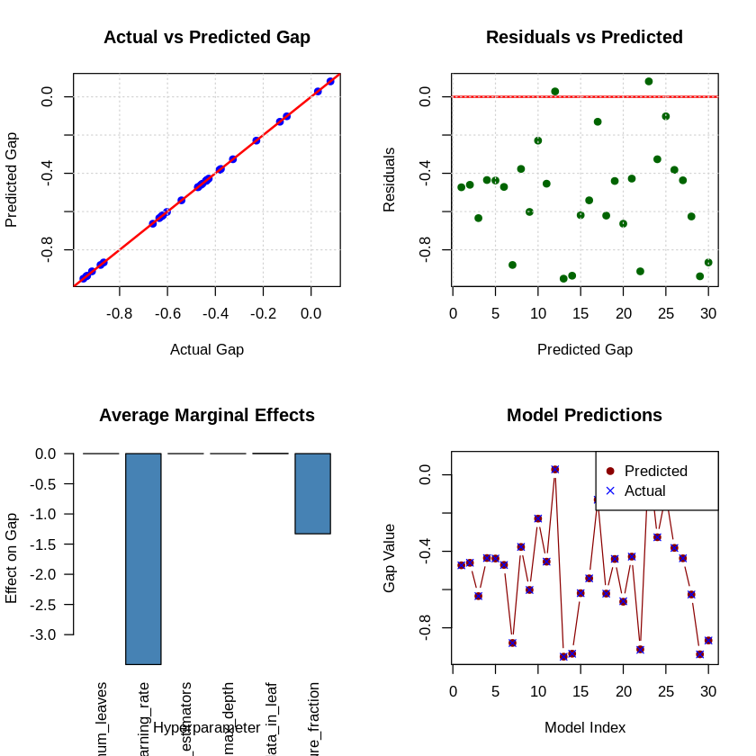
# 6. Diagnostic Plots
cat("\n6. GENERATING DIAGNOSTIC PLOTS...\n")
par(mfrow = c(2, 2))
# Plot 1: Actual vs Predicted
plot(krls_y, krls_model$fitted,
main = "Actual vs Predicted Gap",
xlab = "Actual Gap",
ylab = "Predicted Gap",
pch = 19, col = "blue")
abline(0, 1, col = "red", lwd = 2)
grid()
# Plot 2: Residuals vs Predicted
plot(krls_model$fitted, krls_model$residuals,
main = "Residuals vs Predicted",
xlab = "Predicted Gap",
ylab = "Residuals",
pch = 19, col = "darkgreen")
abline(h = 0, col = "red", lwd = 2)
grid()
# Plot 5: Marginal effects (bar plot)
barplot(partial_derivs,
main = "Average Marginal Effects",
xlab = "Hyperparameter",
ylab = "Effect on Gap",
col = "steelblue",
las = 2)
# Plot 6: Learning curve
plot(krls_model$fitted, type = "b",
main = "Model Predictions",
xlab = "Model Index",
ylab = "Gap Value",
col = "darkred", pch = 19)
points(krls_y, col = "blue", pch = 4)
legend("topright", legend = c("Predicted", "Actual"),
col = c("darkred", "blue"), pch = c(19, 4))
cat(" Diagnostic plots saved to 'krls_diagnostics_r.png'\n")
# 7. Create summary plots of the gap vs hyperparameters
cat("\n7. GAP ANALYSIS BY HYPERPARAMETER:\n")
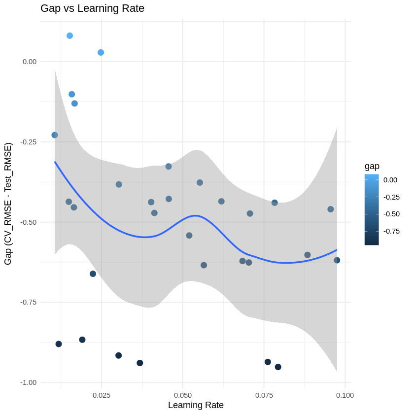
# Plot gap vs learning rate
p1 <- ggplot(results_table, aes(x = learning_rate, y = gap)) +
geom_point(aes(color = gap), size = 3) +
geom_smooth(method = "loess", se = TRUE) +
labs(title = "Gap vs Learning Rate",
x = "Learning Rate",
y = "Gap (CV_RMSE - Test_RMSE)") +
theme_minimal()
print(p1)
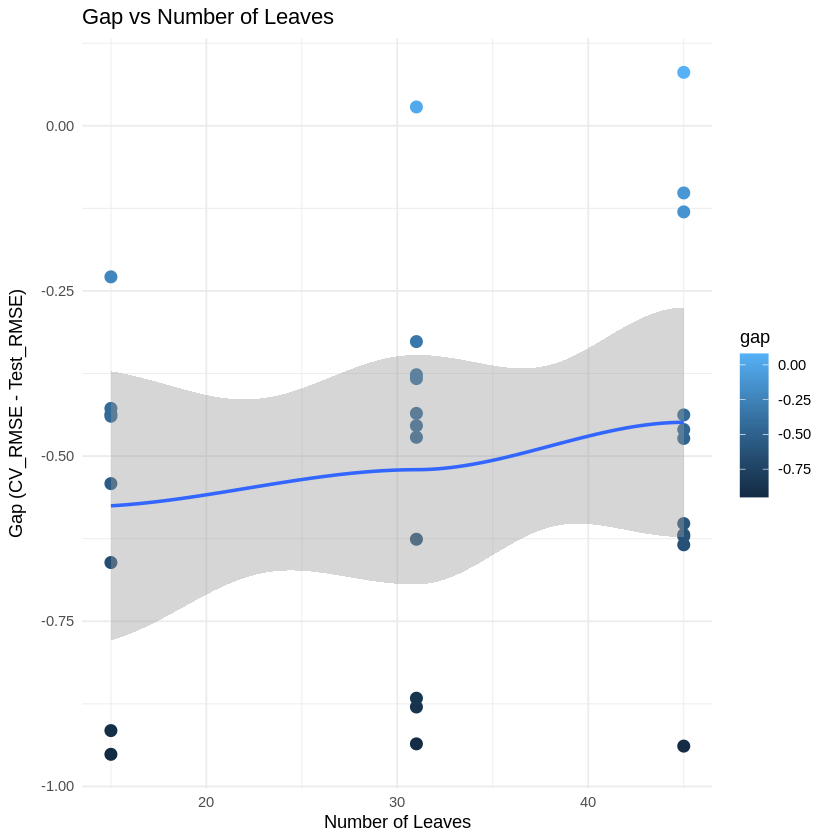
# Plot gap vs num_leaves
p2 <- ggplot(results_table, aes(x = num_leaves, y = gap)) +
geom_point(aes(color = gap), size = 3) +
geom_smooth(method = "loess", se = TRUE) +
labs(title = "Gap vs Number of Leaves",
x = "Number of Leaves",
y = "Gap (CV_RMSE - Test_RMSE)") +
theme_minimal()
print(p2)
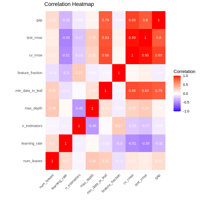
# Plot correlation heatmap
cor_matrix <- cor(results_table[, c("num_leaves", "learning_rate", "n_estimators",
"max_depth", "min_data_in_leaf", "feature_fraction",
"cv_rmse", "test_rmse", "gap")])
p3 <- ggplot(data = reshape2::melt(cor_matrix),
aes(x = Var1, y = Var2, fill = value)) +
geom_tile() +
geom_text(aes(label = round(value, 2)), color = "white", size = 3) +
scale_fill_gradient2(low = "blue", high = "red", mid = "white",
midpoint = 0, limit = c(-1, 1), space = "Lab") +
labs(title = "Correlation Heatmap",
x = "", y = "", fill = "Correlation") +
theme_minimal() +
theme(axis.text.x = element_text(angle = 45, hjust = 1))
print(p3)
# Save gap analysis plots
ggsave("gap_analysis_plots_r.png",
gridExtra::arrangeGrob(p1, p2, p3, ncol = 2),
width = 12, height = 8, dpi = 300)
cat(" Gap analysis plots saved to 'gap_analysis_plots_r.png'\n")
# 8. Find best hyperparameters (lowest gap)
cat("\n8. BEST HYPERPARAMETER CONFIGURATIONS:\n")
# Sort by gap (lowest gap = best generalization)
sorted_results <- results_table[order(abs(results_table$gap)), ]
# Top 3 best configurations
cat("\nTop 3 configurations with smallest gap (best generalization):\n")
for(i in 1:min(3, nrow(sorted_results))) {
cat(paste("\nRank", i, ":\n"))
cat(" Gap:", sorted_results$gap[i], "\n")
cat(" CV RMSE:", sorted_results$cv_rmse[i], "\n")
cat(" Test RMSE:", sorted_results$test_rmse[i], "\n")
cat(" num_leaves:", sorted_results$num_leaves[i], "\n")
cat(" learning_rate:", sorted_results$learning_rate[i], "\n")
cat(" n_estimators:", sorted_results$n_estimators[i], "\n")
cat(" max_depth:", sorted_results$max_depth[i], "\n")
cat(" min_data_in_leaf:", sorted_results$min_data_in_leaf[i], "\n")
cat(" feature_fraction:", sorted_results$feature_fraction[i], "\n")
}
# Worst 3 configurations (largest gap = most overfitting)
sorted_results_worst <- results_table[order(-abs(results_table$gap)), ]
cat("\n\nTop 3 configurations with largest gap (most overfitting):\n")
for(i in 1:min(3, nrow(sorted_results_worst))) {
cat(paste("\nRank", i, ":\n"))
cat(" Gap:", sorted_results_worst$gap[i], "\n")
cat(" CV RMSE:", sorted_results_worst$cv_rmse[i], "\n")
cat(" Test RMSE:", sorted_results_worst$test_rmse[i], "\n")
cat(" num_leaves:", sorted_results_worst$num_leaves[i], "\n")
cat(" learning_rate:", sorted_results_worst$learning_rate[i], "\n")
cat(" n_estimators:", sorted_results_worst$n_estimators[i], "\n")
cat(" max_depth:", sorted_results_worst$max_depth[i], "\n")
cat(" min_data_in_leaf:", sorted_results_worst$min_data_in_leaf[i], "\n")
cat(" feature_fraction:", sorted_results_worst$feature_fraction[i], "\n")
}
# 9. Statistical analysis of gap
cat("\n9. STATISTICAL ANALYSIS OF GAP:\n")
cat(" Mean gap:", mean(results_table$gap), "\n")
cat(" Standard deviation:", sd(results_table$gap), "\n")
cat(" Minimum gap:", min(results_table$gap), "\n")
cat(" Maximum gap:", max(results_table$gap), "\n")
cat(" Median gap:", median(results_table$gap), "\n")
# Test if gap is significantly different from zero
t_test <- t.test(results_table$gap)
cat(" t-test for gap = 0: t =", t_test$statistic,
", p-value =", t_test$p.value, "\n")
if(t_test$p.value < 0.05) {
cat(" Conclusion: Gap is significantly different from zero (p < 0.05)\n")
} else {
cat(" Conclusion: Gap is not significantly different from zero\n")
}
cat("overfitting?")
(t_test2 <- t.test(results_table$gap, alternative = "greater"))
cat("underfitting?")
(t_test3 <- t.test(results_table$gap, alternative = "less"))
# 10. Save KRLS model
saveRDS(krls_model, "krls_model_r.rds")
cat("\n10. KRLS model saved to 'krls_model_r.rds'\n")
cat(paste("\n", paste(rep("=", 80), collapse = ""), "\n"))
cat("ANALYSIS COMPLETE\n")
cat("Results saved to:\n")
cat(" - lightgbm_results_r.csv: LightGBM hyperparameter results\n")
cat(" - krls_model_r.rds: KRLS model object\n")
cat(" - krls_diagnostics_r.png: KRLS diagnostic plots\n")
cat(" - gap_analysis_plots_r.png: Gap analysis visualizations\n")
cat(paste(rep("=", 80), collapse = ""), "\n")
# Print completion message
cat("\n✅ All R code executed successfully!\n")
Training LightGBM models...
Training model 1 of 30 ...
Training model 2 of 30 ...
Training model 3 of 30 ...
Training model 4 of 30 ...
Training model 5 of 30 ...
Training model 6 of 30 ...
Training model 7 of 30 ...
Training model 8 of 30 ...
Training model 9 of 30 ...
Training model 10 of 30 ...
Training model 11 of 30 ...
Training model 12 of 30 ...
Training model 13 of 30 ...
Training model 14 of 30 ...
Training model 15 of 30 ...
Training model 16 of 30 ...
Training model 17 of 30 ...
Training model 18 of 30 ...
Training model 19 of 30 ...
Training model 20 of 30 ...
Training model 21 of 30 ...
Training model 22 of 30 ...
Training model 23 of 30 ...
Training model 24 of 30 ...
Training model 25 of 30 ...
Training model 26 of 30 ...
Training model 27 of 30 ...
Training model 28 of 30 ...
Training model 29 of 30 ...
Training model 30 of 30 ...
================================================================================
FINAL RESULTS TABLE
================================================================================
model_id num_leaves learning_rate n_estimators max_depth min_data_in_leaf
1 1 45 0.07067682 100 10 100
2 2 45 0.09551503 50 10 50
3 3 45 0.05648004 150 -1 20
4 4 31 0.06188671 100 10 100
5 5 45 0.04026981 150 10 100
6 6 31 0.04125922 100 -1 100
7 7 31 0.01180219 150 5 20
8 8 31 0.05525317 150 -1 100
9 9 45 0.08839391 50 5 50
10 10 15 0.01056707 100 5 50
11 11 31 0.01648514 150 -1 50
12 12 31 0.02477901 50 10 100
13 13 15 0.07933007 50 -1 20
14 14 31 0.07616659 150 5 20
15 15 45 0.09746881 100 5 50
16 16 15 0.05198251 150 -1 50
17 17 45 0.01669461 100 5 100
18 18 45 0.06839363 100 -1 50
19 19 15 0.07827339 100 -1 50
20 20 15 0.02233955 50 5 20
21 21 15 0.04569261 100 5 100
22 22 15 0.03024868 50 5 20
23 23 45 0.01521627 50 5 100
24 24 31 0.04563034 50 10 100
25 25 45 0.01584355 100 -1 100
26 26 31 0.03032978 100 -1 100
27 27 15 0.01491662 150 -1 50
28 28 31 0.07032538 150 -1 50
29 29 45 0.03679676 50 10 20
30 30 31 0.01906494 100 5 20
feature_fraction cv_rmse test_rmse gap
1 0.8246258 5.494526 5.967797 -0.47327065
2 0.7622057 4.405432 4.865283 -0.45985065
3 0.7784393 3.508353 4.142610 -0.63425683
4 0.7404175 5.592263 6.027616 -0.43535302
5 0.8705561 5.565326 6.003025 -0.43769840
6 0.8213660 5.619463 6.090962 -0.47149897
7 0.8512196 4.144238 5.023945 -0.87970718
8 0.8125034 5.592810 5.969701 -0.37689099
9 0.7551798 4.306615 4.908771 -0.60215595
10 0.8471117 5.816231 6.044941 -0.22871041
11 0.8098560 4.809378 5.263431 -0.45405362
12 0.7692254 6.704490 6.676068 0.02842218
13 0.8029931 3.585176 4.536517 -0.95134165
14 0.8631536 3.232667 4.168185 -0.93551740
15 0.8052545 4.107878 4.726707 -0.61882871
16 0.7406080 4.294992 4.836629 -0.54163683
17 0.8696215 6.304009 6.434366 -0.13035745
18 0.7740988 4.209949 4.831197 -0.62124727
19 0.7606650 4.308604 4.748225 -0.43962106
20 0.8541194 4.936170 5.597256 -0.66108664
21 0.8466897 5.629371 6.057179 -0.42780729
22 0.8677812 4.276730 5.192173 -0.91544349
23 0.8138098 7.269937 7.189151 0.08078594
24 0.7052562 6.003408 6.330080 -0.32667215
25 0.7972254 6.372935 6.474612 -0.10167741
26 0.8085362 5.826914 6.209579 -0.38266514
27 0.8673320 4.877480 5.314011 -0.43653105
28 0.8457329 4.065288 4.691104 -0.62581641
29 0.8110228 3.989341 4.928279 -0.93893733
30 0.7146829 4.122488 4.988929 -0.86644109
================================================================================
KRLS MODEL DIAGNOSTICS
================================================================================
Fitting KRLS model...
Warning message in Eigenobject$values + lambda:
“Recycling array of length 1 in vector-array arithmetic is deprecated.
Use c() or as.vector() instead.”
Warning message in Eigenobject$values + lambda:
“Recycling array of length 1 in vector-array arithmetic is deprecated.
Use c() or as.vector() instead.”
Average Marginal Effects:
num_leaves learning_rate n_estimators max_depth
-0.0006775316 -3.4958642058 0.0001547258 0.0000539840
min_data_in_leaf feature_fraction
0.0036386780 -1.3287593021
Quartiles of Marginal Effects:
num_leaves learning_rate n_estimators max_depth min_data_in_leaf
25% -0.0060738302 -6.370737 -0.0013469621 -0.011036161 0.002516728
50% 0.0006160114 -3.803870 -0.0003363643 -0.001179409 0.003490419
75% 0.0030558833 1.066097 0.0018319185 0.011030560 0.004452554
feature_fraction
25% -2.1374687
50% -1.0932481
75% -0.5645319
1. MODEL SUMMARY:
* *********************** *
Model Summary:
R2: 0.9999921
Average Marginal Effects:
Est Std. Error t value Pr(>|t|)
num_leaves -0.0006775316 1.571372e-05 -43.117190 2.978229e-24
learning_rate -3.4958642058 1.018814e-02 -343.130816 8.275458e-46
n_estimators 0.0001547258 5.307425e-06 29.152697 3.006099e-20
max_depth 0.0000539840 3.761508e-05 1.435169 1.641438e-01
min_data_in_leaf 0.0036386780 3.869550e-06 940.336222 2.575816e-56
feature_fraction -1.3287593021 6.912165e-03 -192.234897 9.007823e-40
Quartiles of Marginal Effects:
25% 50% 75%
num_leaves -0.006073830 0.0006160114 0.003055883
learning_rate -6.370737399 -3.8038702998 1.066097189
n_estimators -0.001346962 -0.0003363643 0.001831918
max_depth -0.011036161 -0.0011794090 0.011030560
min_data_in_leaf 0.002516728 0.0034904192 0.004452554
feature_fraction -2.137468689 -1.0932481142 -0.564531874
$coefficients
Est Std. Error t value Pr(>|t|)
num_leaves -0.0006775316 1.571372e-05 -43.117190 2.978229e-24
learning_rate -3.4958642058 1.018814e-02 -343.130816 8.275458e-46
n_estimators 0.0001547258 5.307425e-06 29.152697 3.006099e-20
max_depth 0.0000539840 3.761508e-05 1.435169 1.641438e-01
min_data_in_leaf 0.0036386780 3.869550e-06 940.336222 2.575816e-56
feature_fraction -1.3287593021 6.912165e-03 -192.234897 9.007823e-40
$qcoefficients
25% 50% 75%
num_leaves -0.006073830 0.0006160114 0.003055883
learning_rate -6.370737399 -3.8038702998 1.066097189
n_estimators -0.001346962 -0.0003363643 0.001831918
max_depth -0.011036161 -0.0011794090 0.011030560
min_data_in_leaf 0.002516728 0.0034904192 0.004452554
feature_fraction -2.137468689 -1.0932481142 -0.564531874
attr(,"class")
[1] "summary.krls"
2. OPTIMAL HYPERPARAMETERS:
Lambda (regularization): 0.0006817663
Sigma (kernel bandwidth): 6
3. MODEL FIT STATISTICS:
$K
1 2 3 4 5 6
1 1.00000000 0.346289988 0.08604608 0.46583410 0.531980254 0.23136523
2 0.34628999 1.000000000 0.07352161 0.31609701 0.050345647 0.05942486
3 0.08604608 0.073521612 1.00000000 0.07500076 0.069672906 0.19728663
4 0.46583410 0.316097007 0.07500076 1.00000000 0.158483840 0.19829352
5 0.53198025 0.050345647 0.06967291 0.15848384 1.000000000 0.18004778
6 0.23136523 0.059424863 0.19728663 0.19829352 0.180047779 1.00000000
7 0.08353374 0.022254261 0.25312920 0.05563248 0.203463068 0.16867710
8 0.20166404 0.038388360 0.28570968 0.18245112 0.208883011 0.72737054
9 0.27928707 0.794316964 0.16778783 0.28598463 0.042688968 0.13623105
10 0.08435643 0.025334866 0.07646097 0.09968598 0.118803179 0.29117772
11 0.07571185 0.019969536 0.45340554 0.08249890 0.130906958 0.45668559
12 0.30303663 0.178541700 0.02973416 0.52779470 0.121535116 0.20788662
13 0.03534573 0.091144171 0.10269303 0.05488055 0.008439491 0.15630714
14 0.17088805 0.083772785 0.31665779 0.07614689 0.187044632 0.14640795
15 0.46222950 0.537663280 0.31939037 0.24602887 0.149605216 0.19522609
16 0.03635723 0.026874537 0.27745263 0.13590608 0.024263959 0.23786775
17 0.36093089 0.045295447 0.08333074 0.11940040 0.543990304 0.43042775
18 0.20236433 0.226249336 0.64783512 0.17753861 0.079026686 0.39713806
19 0.06312870 0.089130403 0.20781601 0.16601762 0.019673584 0.28888793
20 0.04716451 0.040292828 0.04475880 0.04878997 0.034647311 0.13885161
21 0.23891870 0.051138500 0.05353973 0.24701147 0.207535089 0.51824176
22 0.05135419 0.042290763 0.04223913 0.04349449 0.037121045 0.13527760
23 0.30602606 0.107732374 0.06084093 0.20287629 0.188884536 0.38222406
24 0.18617699 0.248696037 0.02466316 0.65795994 0.036487174 0.09993542
25 0.16981623 0.040955724 0.20057580 0.13782465 0.159003263 0.66063043
26 0.19139045 0.048929561 0.19088522 0.20068332 0.158632956 0.96181365
27 0.02869303 0.004393955 0.11758836 0.02596390 0.074651486 0.28853914
28 0.14412534 0.049949326 0.47996622 0.08149825 0.151951286 0.41913815
29 0.22740404 0.338765962 0.10219614 0.14327313 0.102542010 0.08291039
30 0.05680967 0.098014357 0.24221300 0.19849453 0.029190144 0.11123236
7 8 9 10 11 12
1 0.08353374 0.20166404 0.27928707 0.08435643 0.07571185 0.30303663
2 0.02225426 0.03838836 0.79431696 0.02533487 0.01996954 0.17854170
3 0.25312920 0.28570968 0.16778783 0.07646097 0.45340554 0.02973416
4 0.05563248 0.18245112 0.28598463 0.09968598 0.08249890 0.52779470
5 0.20346307 0.20888301 0.04268897 0.11880318 0.13090696 0.12153512
6 0.16867710 0.72737054 0.13623105 0.29117772 0.45668559 0.20788662
7 1.00000000 0.16775249 0.03243262 0.49742661 0.56402602 0.06322869
8 0.16775249 1.00000000 0.08491953 0.16884237 0.49360692 0.08525776
9 0.03243262 0.08491953 1.00000000 0.03722578 0.05015200 0.17659894
10 0.49742661 0.16884237 0.03722578 1.00000000 0.37379621 0.19447656
11 0.56402602 0.49360692 0.05015200 0.37379621 1.00000000 0.07280995
12 0.06322869 0.08525776 0.17659894 0.19447656 0.07280995 1.00000000
13 0.05635948 0.08648542 0.18849557 0.14706525 0.09126903 0.04824994
14 0.38980010 0.21497344 0.09812921 0.18574599 0.23419492 0.03108749
15 0.08779619 0.20655751 0.62443052 0.05686089 0.10213028 0.09429782
16 0.13554587 0.35174223 0.06469527 0.16595863 0.39418690 0.04950084
17 0.23082770 0.25192233 0.06376506 0.23377337 0.23824100 0.23127387
18 0.12322873 0.36437899 0.49923265 0.08264504 0.30276374 0.09691570
19 0.07414916 0.28703283 0.19320140 0.15123801 0.20180365 0.07260919
20 0.24769163 0.05021887 0.05660321 0.64688483 0.14034912 0.13782273
21 0.17118178 0.37506951 0.06717402 0.52467110 0.21583879 0.26764920
22 0.23070362 0.05051843 0.05711408 0.59495921 0.12234715 0.11406771
23 0.09568708 0.13928907 0.16140138 0.17161395 0.13812536 0.54436559
24 0.01742562 0.05078508 0.24577592 0.05506153 0.03090827 0.67176038
25 0.14039623 0.42253863 0.10441903 0.14859715 0.41712771 0.19942358
26 0.17727198 0.66406842 0.11771286 0.31026727 0.50699701 0.23917213
27 0.46795417 0.28657319 0.01045290 0.54187859 0.58349973 0.02998785
28 0.29679549 0.60679795 0.10174221 0.18681680 0.47411792 0.03407665
29 0.16950689 0.03473544 0.30883491 0.14858424 0.07671845 0.26502233
30 0.19254232 0.08082403 0.16064136 0.17719862 0.25246086 0.19203908
13 14 15 16 17 18
1 0.035345734 0.17088805 0.46222950 0.03635723 0.36093089 0.20236433
2 0.091144171 0.08377278 0.53766328 0.02687454 0.04529545 0.22624934
3 0.102693034 0.31665779 0.31939037 0.27745263 0.08333074 0.64783512
4 0.054880549 0.07614689 0.24602887 0.13590608 0.11940040 0.17753861
5 0.008439491 0.18704463 0.14960522 0.02426396 0.54399030 0.07902669
6 0.156307139 0.14640795 0.19522609 0.23786775 0.43042775 0.39713806
7 0.056359482 0.38980010 0.08779619 0.13554587 0.23082770 0.12322873
8 0.086485422 0.21497344 0.20655751 0.35174223 0.25192233 0.36437899
9 0.188495574 0.09812921 0.62443052 0.06469527 0.06376506 0.49923265
10 0.147065247 0.18574599 0.05686089 0.16595863 0.23377337 0.08264504
11 0.091269028 0.23419492 0.10213028 0.39418690 0.23824100 0.30276374
12 0.048249942 0.03108749 0.09429782 0.04950084 0.23127387 0.09691570
13 1.000000000 0.14261633 0.16114542 0.19014564 0.02311174 0.21669952
14 0.142616329 1.00000000 0.37709671 0.13932554 0.10706054 0.21599740
15 0.161145421 0.37709671 1.00000000 0.09157961 0.11781746 0.56481637
16 0.190145638 0.13932554 0.09157961 1.00000000 0.03059614 0.23418518
17 0.023111738 0.10706054 0.11781746 0.03059614 1.00000000 0.14260731
18 0.216699516 0.21599740 0.56481637 0.23418518 0.14260731 1.00000000
19 0.587162420 0.16898499 0.20619648 0.63542191 0.03202974 0.34113046
20 0.291688463 0.13165649 0.05582112 0.07003192 0.10285788 0.06736485
21 0.147526218 0.17658582 0.11805697 0.16862292 0.28140072 0.10860162
22 0.313634914 0.15791032 0.06431247 0.06029259 0.10114683 0.06575047
23 0.039792623 0.03856414 0.11499272 0.03053815 0.60808968 0.18312776
24 0.039383590 0.01400863 0.08932779 0.05613455 0.05614994 0.09362618
25 0.042489698 0.05597141 0.11297738 0.11023937 0.49934246 0.35780744
26 0.129063909 0.10964327 0.14682185 0.25265479 0.42658081 0.36536614
27 0.086897612 0.20532893 0.03225830 0.22614095 0.13705479 0.07506563
28 0.191193255 0.62363820 0.33592165 0.30667217 0.15548200 0.41802795
29 0.082605104 0.12697780 0.23542668 0.02462642 0.17080283 0.17082390
30 0.104032235 0.07292830 0.09605307 0.27262535 0.05345054 0.22879608
19 20 21 22 23 24 25
1 0.06312870 0.04716451 0.23891870 0.05135419 0.30602606 0.18617699 0.16981623
2 0.08913040 0.04029283 0.05113850 0.04229076 0.10773237 0.24869604 0.04095572
3 0.20781601 0.04475880 0.05353973 0.04223913 0.06084093 0.02466316 0.20057580
4 0.16601762 0.04878997 0.24701147 0.04349449 0.20287629 0.65795994 0.13782465
5 0.01967358 0.03464731 0.20753509 0.03712105 0.18888454 0.03648717 0.15900326
6 0.28888793 0.13885161 0.51824176 0.13527760 0.38222406 0.09993542 0.66063043
7 0.07414916 0.24769163 0.17118178 0.23070362 0.09568708 0.01742562 0.14039623
8 0.28703283 0.05021887 0.37506951 0.05051843 0.13928907 0.05078508 0.42253863
9 0.19320140 0.05660321 0.06717402 0.05711408 0.16140138 0.24577592 0.10441903
10 0.15123801 0.64688483 0.52467110 0.59495921 0.17161395 0.05506153 0.14859715
11 0.20180365 0.14034912 0.21583879 0.12234715 0.13812536 0.03090827 0.41712771
12 0.07260919 0.13782273 0.26764920 0.11406771 0.54436559 0.67176038 0.19942358
13 0.58716242 0.29168846 0.14752622 0.31363491 0.03979262 0.03938359 0.04248970
14 0.16898499 0.13165649 0.17658582 0.15791032 0.03856414 0.01400863 0.05597141
15 0.20619648 0.05582112 0.11805697 0.06431247 0.11499272 0.08932779 0.11297738
16 0.63542191 0.07003192 0.16862292 0.06029259 0.03053815 0.05613455 0.11023937
17 0.03202974 0.10285788 0.28140072 0.10114683 0.60808968 0.05614994 0.49934246
18 0.34113046 0.06736485 0.10860162 0.06575047 0.18312776 0.09362618 0.35780744
19 1.00000000 0.12811529 0.23250392 0.12607833 0.04561090 0.08729144 0.09233471
20 0.12811529 1.00000000 0.26289261 0.97262680 0.12103637 0.04080366 0.06042012
21 0.23250392 0.26289261 1.00000000 0.27374045 0.20250670 0.10576336 0.17727481
22 0.12607833 0.97262680 0.27374045 1.00000000 0.10587179 0.03199563 0.05123700
23 0.04561090 0.12103637 0.20250670 0.10587179 1.00000000 0.22003748 0.54950698
24 0.08729144 0.04080366 0.10576336 0.03199563 0.22003748 1.00000000 0.09473493
25 0.09233471 0.06042012 0.17727481 0.05123700 0.54950698 0.09473493 1.00000000
26 0.25965784 0.13780613 0.46501186 0.12586172 0.42382255 0.11704748 0.75342141
27 0.13457913 0.21405456 0.30415123 0.20820922 0.04969150 0.00731568 0.13042827
28 0.32979054 0.09678693 0.25197916 0.10979976 0.06484106 0.01711810 0.18219854
29 0.04708646 0.23722230 0.07608147 0.22281049 0.28327161 0.13463036 0.09406100
30 0.18607513 0.13634296 0.06897490 0.09912534 0.11535266 0.20396861 0.13817054
26 27 28 29 30
1 0.19139045 0.028693033 0.14412534 0.22740404 0.05680967
2 0.04892956 0.004393955 0.04994933 0.33876596 0.09801436
3 0.19088522 0.117588358 0.47996622 0.10219614 0.24221300
4 0.20068332 0.025963899 0.08149825 0.14327313 0.19849453
5 0.15863296 0.074651486 0.15195129 0.10254201 0.02919014
6 0.96181365 0.288539142 0.41913815 0.08291039 0.11123236
7 0.17727198 0.467954170 0.29679549 0.16950689 0.19254232
8 0.66406842 0.286573190 0.60679795 0.03473544 0.08082403
9 0.11771286 0.010452896 0.10174221 0.30883491 0.16064136
10 0.31026727 0.541878589 0.18681680 0.14858424 0.17719862
11 0.50699701 0.583499728 0.47411792 0.07671845 0.25246086
12 0.23917213 0.029987846 0.03407665 0.26502233 0.19203908
13 0.12906391 0.086897612 0.19119325 0.08260510 0.10403223
14 0.10964327 0.205328927 0.62363820 0.12697780 0.07292830
15 0.14682185 0.032258304 0.33592165 0.23542668 0.09605307
16 0.25265479 0.226140952 0.30667217 0.02462642 0.27262535
17 0.42658081 0.137054791 0.15548200 0.17080283 0.05345054
18 0.36536614 0.075065626 0.41802795 0.17082390 0.22879608
19 0.25965784 0.134579132 0.32979054 0.04708646 0.18607513
20 0.13780613 0.214054560 0.09678693 0.23722230 0.13634296
21 0.46501186 0.304151229 0.25197916 0.07608147 0.06897490
22 0.12586172 0.208209224 0.10979976 0.22281049 0.09912534
23 0.42382255 0.049691497 0.06484106 0.28327161 0.11535266
24 0.11704748 0.007315680 0.01711810 0.13463036 0.20396861
25 0.75342141 0.130428273 0.18219854 0.09406100 0.13817054
26 1.00000000 0.289716118 0.33379602 0.08311499 0.14584314
27 0.28971612 1.000000000 0.36039034 0.02655176 0.06592102
28 0.33379602 0.360390335 1.00000000 0.05985102 0.07721934
29 0.08311499 0.026551763 0.05985102 1.00000000 0.23185448
30 0.14584314 0.065921022 0.07721934 0.23185448 1.00000000
$coeffs
[,1]
[1,] -0.7138638
[2,] 1.7899866
[3,] 0.1927768
[4,] -0.5532582
[5,] 0.1941038
[6,] -1.4142678
[7,] -2.6543658
[8,] 1.7508142
[9,] -1.1009789
[10,] 2.3333399
[11,] 1.3515547
[12,] 2.2094337
[13,] -2.0909906
[14,] -0.4938505
[15,] 0.4587227
[16,] -1.5901434
[17,] 0.7368818
[18,] -0.3543444
[19,] 3.0886970
[20,] 13.9493343
[21,] 0.0591846
[22,] -15.0397146
[23,] 1.4393512
[24,] -0.3981617
[25,] 2.3468539
[26,] -2.8810285
[27,] 0.2784308
[28,] -0.2658538
[29,] -2.1023006
[30,] -1.6524928
$Looe
[,1]
[1,] 3.114752
$fitted
[,1]
1 -0.47313641
2 -0.46018724
3 -0.63429308
4 -0.43524898
5 -0.43773490
6 -0.47123303
7 -0.87920805
8 -0.37722021
9 -0.60194892
10 -0.22914917
11 -0.45430777
12 0.02800671
13 -0.95094846
14 -0.93542454
15 -0.61891497
16 -0.54133782
17 -0.13049601
18 -0.62118064
19 -0.44020187
20 -0.66370969
21 -0.42781842
22 -0.91261541
23 0.08051529
24 -0.32659728
25 -0.10211872
26 -0.38212339
27 -0.43658341
28 -0.62576642
29 -0.93854201
30 -0.86613036
$X
num_leaves learning_rate n_estimators max_depth min_data_in_leaf
[1,] 45 0.07067682 100 10 100
[2,] 45 0.09551503 50 10 50
[3,] 45 0.05648004 150 -1 20
[4,] 31 0.06188671 100 10 100
[5,] 45 0.04026981 150 10 100
[6,] 31 0.04125922 100 -1 100
[7,] 31 0.01180219 150 5 20
[8,] 31 0.05525317 150 -1 100
[9,] 45 0.08839391 50 5 50
[10,] 15 0.01056707 100 5 50
[11,] 31 0.01648514 150 -1 50
[12,] 31 0.02477901 50 10 100
[13,] 15 0.07933007 50 -1 20
[14,] 31 0.07616659 150 5 20
[15,] 45 0.09746881 100 5 50
[16,] 15 0.05198251 150 -1 50
[17,] 45 0.01669461 100 5 100
[18,] 45 0.06839363 100 -1 50
[19,] 15 0.07827339 100 -1 50
[20,] 15 0.02233955 50 5 20
[21,] 15 0.04569261 100 5 100
[22,] 15 0.03024868 50 5 20
[23,] 45 0.01521627 50 5 100
[24,] 31 0.04563034 50 10 100
[25,] 45 0.01584355 100 -1 100
[26,] 31 0.03032978 100 -1 100
[27,] 15 0.01491662 150 -1 50
[28,] 31 0.07032538 150 -1 50
[29,] 45 0.03679676 50 10 20
[30,] 31 0.01906494 100 5 20
feature_fraction
[1,] 0.8246258
[2,] 0.7622057
[3,] 0.7784393
[4,] 0.7404175
[5,] 0.8705561
[6,] 0.8213660
[7,] 0.8512196
[8,] 0.8125034
[9,] 0.7551798
[10,] 0.8471117
[11,] 0.8098560
[12,] 0.7692254
[13,] 0.8029931
[14,] 0.8631536
[15,] 0.8052545
[16,] 0.7406080
[17,] 0.8696215
[18,] 0.7740988
[19,] 0.7606650
[20,] 0.8541194
[21,] 0.8466897
[22,] 0.8677812
[23,] 0.8138098
[24,] 0.7052562
[25,] 0.7972254
[26,] 0.8085362
[27,] 0.8673320
[28,] 0.8457329
[29,] 0.8110228
[30,] 0.7146829
$y
[,1]
[1,] -0.47327065
[2,] -0.45985065
[3,] -0.63425683
[4,] -0.43535302
[5,] -0.43769840
[6,] -0.47149897
[7,] -0.87970718
[8,] -0.37689099
[9,] -0.60215595
[10,] -0.22871041
[11,] -0.45405362
[12,] 0.02842218
[13,] -0.95134165
[14,] -0.93551740
[15,] -0.61882871
[16,] -0.54163683
[17,] -0.13035745
[18,] -0.62124727
[19,] -0.43962106
[20,] -0.66108664
[21,] -0.42780729
[22,] -0.91544349
[23,] 0.08078594
[24,] -0.32667215
[25,] -0.10167741
[26,] -0.38266514
[27,] -0.43653105
[28,] -0.62581641
[29,] -0.93893733
[30,] -0.86644109
$sigma
[1] 6
$lambda
[,1]
[1,] 0.0006817663
$R2
[,1]
[1,] 0.9999921
$derivatives
num_leaves learning_rate n_estimators max_depth min_data_in_leaf
[1,] 1.466634e-03 -3.91848727 -0.0014837374 -0.0048548837 0.0033288224
[2,] 1.952469e-03 4.78968673 -0.0007401287 0.0206455422 0.0030324067
[3,] 5.819306e-03 1.08513623 0.0022512588 -0.0330900165 0.0035415503
[4,] -1.009628e-03 -3.21963314 -0.0029543239 0.0006901616 0.0020033751
[5,] 1.873337e-03 -3.64769308 -0.0013601104 -0.0145351414 0.0041366143
[6,] 9.379902e-03 -6.37372085 0.0020946537 0.0262232220 0.0013726113
[7,] -9.289843e-03 -6.70108654 -0.0009177923 -0.0223401580 0.0066131584
[8,] 4.738914e-03 -1.41260681 0.0024092752 -0.0004274860 0.0010590804
[9,] 3.056838e-03 4.24885061 -0.0002210989 0.0209612193 0.0039592013
[10,] -1.114425e-02 -12.21406207 -0.0025210637 0.0061015727 0.0058590933
[11,] 5.481047e-04 -3.97942649 -0.0004914069 -0.0215230723 0.0060987822
[12,] -1.961513e-04 -6.41720401 -0.0012996865 -0.0100783752 0.0027662047
[13,] -8.114291e-03 1.37902296 0.0028241154 -0.0199188869 0.0031928470
[14,] 1.363518e-03 6.03273331 0.0042100759 -0.0094267820 0.0030486752
[15,] 5.222021e-03 5.55833895 0.0010437128 0.0047934290 0.0034254911
[16,] -4.198528e-03 3.32916677 -0.0013075171 -0.0113554226 0.0024335689
[17,] 3.053019e-03 -5.97011913 -0.0021140404 -0.0019313320 0.0042235195
[18,] 4.964972e-03 0.07300528 0.0025377603 -0.0168740276 0.0045288982
[19,] -8.020141e-03 3.26985802 0.0022986583 -0.0074561140 0.0034392881
[20,] -1.266259e-02 -20.01947459 0.0007305896 0.0091392721 0.0058191864
[21,] -1.849531e-03 -7.70650178 0.0007906704 0.0215267317 0.0019649822
[22,] -1.224125e-02 -19.09425196 0.0007103946 0.0101466014 0.0051524511
[23,] -2.943899e-03 -6.36178706 0.0009000596 0.0124694123 0.0039581927
[24,] -9.088437e-05 -4.02948495 -0.0019004744 0.0039816771 0.0021494519
[25,] 9.896435e-03 -5.56200513 -0.0004516296 0.0313928086 0.0016025581
[26,] 1.081062e-02 -7.15146536 0.0010260161 0.0342898434 0.0005407147
[27,] -6.698931e-03 -5.06452614 -0.0006020958 -0.0042421068 0.0035933148
[28,] 6.839180e-04 1.00898006 0.0035186938 -0.0279919453 0.0052017509
[29,] 1.026719e-03 -3.68925333 -0.0023793391 0.0113252134 0.0071126569
[30,] -7.722759e-03 -3.11791542 -0.0019597167 -0.0060214366 0.0040018918
feature_fraction
[1,] -1.130705914
[2,] -1.333755975
[3,] -0.560086679
[4,] 1.639316837
[5,] -0.761448884
[6,] -1.436435039
[7,] -1.055790315
[8,] -0.577867459
[9,] -1.343874436
[10,] -4.146393405
[11,] -0.004762551
[12,] 2.330924021
[13,] -5.514804447
[14,] -0.971536878
[15,] -1.924830440
[16,] 1.670745806
[17,] -3.560164436
[18,] -0.798497972
[19,] -2.287127860
[20,] -6.861491470
[21,] -2.852144134
[22,] -6.420371092
[23,] -1.049280231
[24,] 3.796480779
[25,] 0.611629791
[26,] -0.678785223
[27,] -1.817482076
[28,] -2.208348106
[29,] -1.688102670
[30,] 1.072211395
$avgderivatives
num_leaves learning_rate n_estimators max_depth min_data_in_leaf
[1,] -0.0006775316 -3.495864 0.0001547258 5.3984e-05 0.003638678
feature_fraction
[1,] -1.328759
$var.avgderivatives
num_leaves learning_rate n_estimators max_depth min_data_in_leaf
[1,] 2.469211e-10 0.0001037982 2.816876e-11 1.414894e-09 1.497342e-11
feature_fraction
[1,] 4.777802e-05
$vcov.c
[,1] [,2] [,3] [,4] [,5]
[1,] 7.198390e-06 -2.176901e-06 -2.707928e-07 -3.939010e-06 -4.491910e-06
[2,] -2.176901e-06 1.450342e-05 -4.479936e-06 -5.349111e-07 1.007133e-06
[3,] -2.707928e-07 -4.479936e-06 7.331466e-06 5.334838e-07 5.249473e-07
[4,] -3.939010e-06 -5.349111e-07 5.334838e-07 5.675790e-06 1.925799e-06
[5,] -4.491910e-06 1.007133e-06 5.249473e-07 1.925799e-06 5.276935e-06
...
$vcov.fitted
1 2 3 4 5
1 5.770597e-07 3.586715e-10 -4.683216e-11 7.280141e-10 8.245260e-10
2 3.586715e-10 5.761571e-07 3.452175e-10 1.418792e-10 -1.615939e-10
3 -4.683216e-11 3.452175e-10 5.769929e-07 -2.115664e-11 -1.518574e-11
4 7.280141e-10 1.418792e-10 -2.115664e-11 5.770635e-07 -1.658241e-10
5 8.245260e-10 -1.615939e-10 -1.518574e-11 -1.658241e-10 5.773684e-07
...
$binaryindicator
num_leaves learning_rate n_estimators max_depth min_data_in_leaf
[1,] FALSE FALSE FALSE FALSE FALSE
feature_fraction
[1,] FALSE
attr(,"class")
[1] "krls"
4. PARTIAL DERIVATIVES (Average Marginal Effects):
num_leaves learning_rate n_estimators max_depth
-0.0006775316 -3.4958642058 0.0001547258 0.0000539840
min_data_in_leaf feature_fraction
0.0036386780 -1.3287593021
6. GENERATING DIAGNOSTIC PLOTS...
Diagnostic plots saved to 'krls_diagnostics_r.png'
7. GAP ANALYSIS BY HYPERPARAMETER:
[1m[22m`geom_smooth()` using formula = 'y ~ x'
[1m[22m`geom_smooth()` using formula = 'y ~ x'
Warning message in simpleLoess(y, x, w, span, degree = degree, parametric = parametric, :
“pseudoinverse used at 14.85”
Warning message in simpleLoess(y, x, w, span, degree = degree, parametric = parametric, :
“neighborhood radius 30.15”
Warning message in simpleLoess(y, x, w, span, degree = degree, parametric = parametric, :
“reciprocal condition number 4.5167e-17”
Warning message in simpleLoess(y, x, w, span, degree = degree, parametric = parametric, :
“There are other near singularities as well. 200.22”
Warning message in predLoess(object$y, object$x, newx = if (is.null(newdata)) object$x else if (is.data.frame(newdata)) as.matrix(model.frame(delete.response(terms(object)), :
“pseudoinverse used at 14.85”
Warning message in predLoess(object$y, object$x, newx = if (is.null(newdata)) object$x else if (is.data.frame(newdata)) as.matrix(model.frame(delete.response(terms(object)), :
“neighborhood radius 30.15”
Warning message in predLoess(object$y, object$x, newx = if (is.null(newdata)) object$x else if (is.data.frame(newdata)) as.matrix(model.frame(delete.response(terms(object)), :
“reciprocal condition number 4.5167e-17”
Warning message in predLoess(object$y, object$x, newx = if (is.null(newdata)) object$x else if (is.data.frame(newdata)) as.matrix(model.frame(delete.response(terms(object)), :
“There are other near singularities as well. 200.22”
[1m[22m`geom_smooth()` using formula = 'y ~ x'
[1m[22m`geom_smooth()` using formula = 'y ~ x'
Warning message in simpleLoess(y, x, w, span, degree = degree, parametric = parametric, :
“pseudoinverse used at 14.85”
Warning message in simpleLoess(y, x, w, span, degree = degree, parametric = parametric, :
“neighborhood radius 30.15”
Warning message in simpleLoess(y, x, w, span, degree = degree, parametric = parametric, :
“reciprocal condition number 4.5167e-17”
Warning message in simpleLoess(y, x, w, span, degree = degree, parametric = parametric, :
“There are other near singularities as well. 200.22”
Warning message in predLoess(object$y, object$x, newx = if (is.null(newdata)) object$x else if (is.data.frame(newdata)) as.matrix(model.frame(delete.response(terms(object)), :
“pseudoinverse used at 14.85”
Warning message in predLoess(object$y, object$x, newx = if (is.null(newdata)) object$x else if (is.data.frame(newdata)) as.matrix(model.frame(delete.response(terms(object)), :
“neighborhood radius 30.15”
Warning message in predLoess(object$y, object$x, newx = if (is.null(newdata)) object$x else if (is.data.frame(newdata)) as.matrix(model.frame(delete.response(terms(object)), :
“reciprocal condition number 4.5167e-17”
Warning message in predLoess(object$y, object$x, newx = if (is.null(newdata)) object$x else if (is.data.frame(newdata)) as.matrix(model.frame(delete.response(terms(object)), :
“There are other near singularities as well. 200.22”
Gap analysis plots saved to 'gap_analysis_plots_r.png'
8. BEST HYPERPARAMETER CONFIGURATIONS:
Top 3 configurations with smallest gap (best generalization):
Rank 1 :
Gap: 0.02842218
CV RMSE: 6.70449
Test RMSE: 6.676068
num_leaves: 31
learning_rate: 0.02477901
n_estimators: 50
max_depth: 10
min_data_in_leaf: 100
feature_fraction: 0.7692254
Rank 2 :
Gap: 0.08078594
CV RMSE: 7.269937
Test RMSE: 7.189151
num_leaves: 45
learning_rate: 0.01521627
n_estimators: 50
max_depth: 5
min_data_in_leaf: 100
feature_fraction: 0.8138098
Rank 3 :
Gap: -0.1016774
CV RMSE: 6.372935
Test RMSE: 6.474612
num_leaves: 45
learning_rate: 0.01584355
n_estimators: 100
max_depth: -1
min_data_in_leaf: 100
feature_fraction: 0.7972254
Top 3 configurations with largest gap (most overfitting):
Rank 1 :
Gap: -0.9513416
CV RMSE: 3.585176
Test RMSE: 4.536517
num_leaves: 15
learning_rate: 0.07933007
n_estimators: 50
max_depth: -1
min_data_in_leaf: 20
feature_fraction: 0.8029931
Rank 2 :
Gap: -0.9389373
CV RMSE: 3.989341
Test RMSE: 4.928279
num_leaves: 45
learning_rate: 0.03679676
n_estimators: 50
max_depth: 10
min_data_in_leaf: 20
feature_fraction: 0.8110228
Rank 3 :
Gap: -0.9355174
CV RMSE: 3.232667
Test RMSE: 4.168185
num_leaves: 31
learning_rate: 0.07616659
n_estimators: 150
max_depth: 5
min_data_in_leaf: 20
feature_fraction: 0.8631536
9. STATISTICAL ANALYSIS OF GAP:
Mean gap: -0.5088622
Standard deviation: 0.2758146
Minimum gap: -0.9513416
Maximum gap: 0.08078594
Median gap: -0.4656748
t-test for gap = 0: t = -10.10517 , p-value = 5.20261e-11
Conclusion: Gap is significantly different from zero (p < 0.05)
overfitting?
One Sample t-test
data: results_table$gap
t = -10.105, df = 29, p-value = 1
alternative hypothesis: true mean is greater than 0
95 percent confidence interval:
-0.5944245 Inf
sample estimates:
mean of x
-0.5088622
underfitting?
One Sample t-test
data: results_table$gap
t = -10.105, df = 29, p-value = 2.601e-11
alternative hypothesis: true mean is less than 0
95 percent confidence interval:
-Inf -0.4232999
sample estimates:
mean of x
-0.5088622
✅ All R code executed successfully!
For attribution, please cite this work as:
T. Moudiki (2026-01-25). Beyond Cross-validation: Hyperparameter Optimization via Generalization Gap Modeling. Retrieved from https://thierrymoudiki.github.io/blog/2026/01/25/r/gap-modeling-in-R
BibTeX citation (remove empty spaces)
        @misc{ tmoudiki20260125,
          author = { T. Moudiki },
          title = { Beyond Cross-validation: Hyperparameter Optimization via Generalization Gap Modeling },
          url = { https://thierrymoudiki.github.io/blog/2026/01/25/r/gap-modeling-in-R },
          year = { 2026 } }

Previous publications
- GPopt for R: Bayesian and conformal optimization of black-box functions and hyperparameter tuning Jul 26, 2026
- My last R posts: How conformalization helps weak models, fast conformal prediction with jackknife+ (and no refitting), and sklearn in R Jul 13, 2026
- Natively Interpretable Boosting Jul 12, 2026
- Fast conformal prediction (no refitting) for some Machine Learning models via closed-form jackknife plus Jun 27, 2026
- Using scikit-learn models in R easily with the tisthemachinelearner package Jun 21, 2026
- No-Code Machine Learning in Excel with the Techtonique API Jun 14, 2026
- How Conformal Prediction Makes Linear Models Good Enough — An Example Using R Package mlS3 Jun 7, 2026
- Techtonique dot net, the Machine Learning web API, is back online (but more like a passion project for now) May 31, 2026
- Conformalized TabICL: Prediction Intervals for a State-Of-The-Art Tabular Foundation Model in Python and R May 21, 2026
- Conformalized TabPFN: Prediction Intervals for a Pretrained Transformer for Tabular Data in Python and R May 17, 2026
- Probabilistic Time Series Cross-Validation with R package crossvalidation May 16, 2026
- One interface, (Almost) Every Classifier (and Regressor): unifiedml v0.3.0 May 9, 2026
- You Don't Need to Learn All the Weights on tabular data: The Case for rvflnet (a nonlinear expressive glmnet) on regression, classification and survival analysis May 2, 2026
- Survival analysis with sklearn, glmnet, keras, pytorch, lightgbm, xgboost, nnetsauce, mlsauce Part 2 Apr 28, 2026
- Any Sklearn Regressor as a Survival Model — Does It Actually Work? Benchmarking vs Established Packages Apr 26, 2026
- Conformal Optimization Beats Bayesian Optimization, Optuna and Random Search on 72 classification Datasets Apr 19, 2026
- `mlS3` — A Unified S3 Machine Learning Interface in R Apr 12, 2026
- One interface, (Almost) Every Classifier: unifiedml v0.2.1 Apr 4, 2026
- Techtonique dot net is down until further notice Apr 1, 2026
- Explaining Time-Series Forecasts with Sensitivity Analysis (ahead::dynrmf and external regressors) Mar 29, 2026
- Python version of 'Option pricing using time series models as market price of risk Pt.3' Mar 22, 2026
- Option pricing using time series models as market price of risk Pt.3 Mar 16, 2026
- Explaining Time-Series Forecasts with Exact Shapley Values (ahead::dynrmf with external regressors applied to scenarios) Mar 8, 2026
- My Presentation at Risk 2026: Lightweight Transfer Learning for Financial Forecasting Mar 1, 2026
- nnetsauce with and without jax for GPU acceleration Feb 23, 2026
- Understanding Boosted Configuration Networks (combined neural networks and boosting): An Intuitive Guide Through Their Hyperparameters Feb 16, 2026
- R version of Python package survivalist, for model-agnostic survival analysis Feb 9, 2026
- Presenting Lightweight Transfer Learning for Financial Forecasting (Risk 2026) Feb 4, 2026
- Option pricing using time series models as market price of risk Feb 1, 2026
- Enhancing Time Series Forecasting (ahead::ridge2f) with Attention-Based Context Vectors (ahead::contextridge2f) Jan 31, 2026
- Overfitting and scaling (on GPU T4) tests on nnetsauce.CustomRegressor Jan 29, 2026
- Beyond Cross-validation: Hyperparameter Optimization via Generalization Gap Modeling Jan 25, 2026
- GPopt for Machine Learning (hyperparameters' tuning) Jan 21, 2026
- rtopy: an R to Python bridge -- novelties Jan 8, 2026
- Python examples for 'Beyond Nelson-Siegel and splines: A model- agnostic Machine Learning framework for discount curve calibration, interpolation and extrapolation' Jan 3, 2026
- Forecasting benchmark: Dynrmf (a new serious competitor in town) vs Theta Method on M-Competitions and Tourism competitition Jan 1, 2026
- Finally figured out a way to port python packages to R using uv and reticulate: example with nnetsauce Dec 17, 2025
- Overfitting Random Fourier Features: Universal Approximation Property Dec 13, 2025
- Counterfactual Scenario Analysis with ahead::ridge2f Dec 11, 2025
- Zero-Shot Probabilistic Time Series Forecasting with TabPFN 2.5 and nnetsauce Dec 10, 2025
- ARIMA Pricing: Semi-Parametric Market price of risk for Risk-Neutral Pricing (code + preprint) Dec 7, 2025
- Analyzing Paper Reviews with LLMs: I Used ChatGPT, DeepSeek, Qwen, Mistral, Gemini, and Claude (and you should too + publish the analysis) Dec 3, 2025
- tisthemachinelearner: New Workflow with uv for R Integration of scikit-learn Dec 1, 2025
- (ICYMI) RPweave: Unified R + Python + LaTeX System using uv Nov 21, 2025
- unifiedml: A Unified Machine Learning Interface for R, is now on CRAN + Discussion about AI replacing humans Nov 16, 2025
- Context-aware Theta forecasting Method: Extending Classical Time Series Forecasting with Machine Learning Nov 13, 2025
- unifiedml in R: A Unified Machine Learning Interface Nov 5, 2025
- Deterministic Shift Adjustment in Arbitrage-Free Pricing (historical to risk-neutral short rates) Oct 28, 2025
- New instantaneous short rates models with their deterministic shift adjustment, for historical and risk-neutral simulation Oct 27, 2025
- RPweave: Unified R + Python + LaTeX System using uv Oct 19, 2025
- GAN-like Synthetic Data Generation Examples (on univariate, multivariate distributions, digits recognition, Fashion-MNIST, stock returns, and Olivetti faces) with DistroSimulator Oct 19, 2025
- R port of llama2.c Oct 9, 2025
- Native uncertainty quantification for time series with NGBoost Oct 8, 2025
- NGBoost (Natural Gradient Boosting) for Regression, Classification, Time Series forecasting and Reserving Oct 6, 2025
- Real-time pricing with a pretrained probabilistic stock return model Oct 1, 2025
- Combining any model with GARCH(1,1) for probabilistic stock forecasting Sep 23, 2025
- Generating Synthetic Data with R-vine Copulas using esgtoolkit in R Sep 21, 2025
- Reimagining Equity Solvency Capital Requirement Approximation (one of my Master's Thesis subjects): From Bilinear Interpolation to Probabilistic Machine Learning Sep 16, 2025
- Transfer Learning using ahead::ridge2f on synthetic stocks returns Pt.2: synthetic data generation Sep 9, 2025
- Transfer Learning using ahead::ridge2f on synthetic stocks returns Sep 8, 2025
- I'm supposed to present 'Conformal Predictive Simulations for Univariate Time Series' at COPA CONFERENCE 2025 in London... Sep 4, 2025
- external regressors in ahead::dynrmf's interface for Machine learning forecasting Sep 1, 2025
- Another interesting decision, now for 'Beyond Nelson-Siegel and splines: A model-agnostic Machine Learning framework for discount curve calibration, interpolation and extrapolation' Aug 20, 2025
- Boosting any randomized based learner for regression, classification and univariate/multivariate time series forcasting Jul 26, 2025
- New nnetsauce version with CustomBackPropRegressor (CustomRegressor with Backpropagation) and ElasticNet2Regressor (Ridge2 with ElasticNet regularization) Jul 15, 2025
- mlsauce (home to a model-agnostic gradient boosting algorithm) can now be installed from PyPI. Jul 10, 2025
- A user-friendly graphical interface to techtonique dot net's API (will eventually contain graphics). Jul 8, 2025
- Calling =TECHTO_MLCLASSIFICATION for Machine Learning supervised CLASSIFICATION in Excel is just a matter of copying and pasting Jul 7, 2025
- Calling =TECHTO_MLREGRESSION for Machine Learning supervised regression in Excel is just a matter of copying and pasting Jul 6, 2025
- Calling =TECHTO_RESERVING and =TECHTO_MLRESERVING for claims triangle reserving in Excel is just a matter of copying and pasting Jul 5, 2025
- Calling =TECHTO_SURVIVAL for Survival Analysis in Excel is just a matter of copying and pasting Jul 4, 2025
- Calling =TECHTO_SIMULATION for Stochastic Simulation in Excel is just a matter of copying and pasting Jul 3, 2025
- Calling =TECHTO_FORECAST for forecasting in Excel is just a matter of copying and pasting Jul 2, 2025
- Random Vector Functional Link (RVFL) artificial neural network with 2 regularization parameters successfully used for forecasting/synthetic simulation in professional settings: Extensions (including Bayesian) Jul 1, 2025
- R version of 'Backpropagating quasi-randomized neural networks' Jun 24, 2025
- Backpropagating quasi-randomized neural networks Jun 23, 2025
- Beyond ARMA-GARCH: leveraging any statistical model for volatility forecasting Jun 21, 2025
- Stacked generalization (Machine Learning model stacking) + conformal prediction for forecasting with ahead::mlf Jun 18, 2025
- An Overfitting dilemma: XGBoost Default Hyperparameters vs GenericBooster + LinearRegression Default Hyperparameters Jun 14, 2025
- Programming language-agnostic reserving using RidgeCV, LightGBM, XGBoost, and ExtraTrees Machine Learning models Jun 13, 2025
- Free R, Python and SQL editors in techtonique dot net Jun 9, 2025
- Beyond Nelson-Siegel and splines: A model-agnostic Machine Learning framework for discount curve calibration, interpolation and extrapolation Jun 7, 2025
- scikit-learn, glmnet, xgboost, lightgbm, pytorch, keras, nnetsauce in probabilistic Machine Learning (for longitudinal data) Reserving (work in progress) Jun 6, 2025
- R version of Probabilistic Machine Learning (for longitudinal data) Reserving (work in progress) Jun 5, 2025
- Probabilistic Machine Learning (for longitudinal data) Reserving (work in progress) Jun 4, 2025
- Python version of Beyond ARMA-GARCH: leveraging model-agnostic Quasi-Randomized networks and conformal prediction for nonparametric probabilistic stock forecasting (ML-ARCH) Jun 3, 2025
- Beyond ARMA-GARCH: leveraging model-agnostic Machine Learning and conformal prediction for nonparametric probabilistic stock forecasting (ML-ARCH) Jun 2, 2025
- Permutations and SHAPley values for feature importance in techtonique dot net's API (with R + Python + the command line) Jun 1, 2025
- Which patient is going to survive longer? Another guide to using techtonique dot net's API (with R + Python + the command line) for survival analysis May 31, 2025
- A Guide to Using techtonique.net's API and rush for simulating and plotting Stochastic Scenarios May 30, 2025
- Simulating Stochastic Scenarios with Diffusion Models: A Guide to Using techtonique.net's API for the purpose May 29, 2025
- Will my apartment in 5th avenue be overpriced or not? Harnessing the power of www.techtonique.net (+ xgboost, lightgbm, catboost) to find out May 28, 2025
- How long must I wait until something happens: A Comprehensive Guide to Survival Analysis via an API May 27, 2025
- Harnessing the Power of techtonique.net: A Comprehensive Guide to Machine Learning Classification via an API May 26, 2025
- Quantile regression with any regressor -- Examples with RandomForestRegressor, RidgeCV, KNeighborsRegressor May 20, 2025
- Survival stacking: survival analysis translated as supervised classification in R and Python May 5, 2025
- 'Bayesian' optimization of hyperparameters in a R machine learning model using the bayesianrvfl package Apr 25, 2025
- A lightweight interface to scikit-learn in R: Bayesian and Conformal prediction Apr 21, 2025
- A lightweight interface to scikit-learn in R Pt.2: probabilistic time series forecasting in conjunction with ahead::dynrmf Apr 20, 2025
- Extending the Theta forecasting method to GLMs, GAMs, GLMBOOST and attention: benchmarking on Tourism, M1, M3 and M4 competition data sets (28000 series) Apr 14, 2025
- Extending the Theta forecasting method to GLMs and attention Apr 8, 2025
- Nonlinear conformalized Generalized Linear Models (GLMs) with R package 'rvfl' (and other models) Mar 31, 2025
- Probabilistic Time Series Forecasting (predictive simulations) in Microsoft Excel using Python, xlwings lite and www.techtonique.net Mar 28, 2025
- Conformalize (improved prediction intervals and simulations) any R Machine Learning model with misc::conformalize Mar 25, 2025
- My poster for the 18th FINANCIAL RISKS INTERNATIONAL FORUM by Institut Louis Bachelier/Fondation du Risque/Europlace Institute of Finance Mar 19, 2025
- Interpretable probabilistic kernel ridge regression using Matérn 3/2 kernels Mar 16, 2025
- (News from) Probabilistic Forecasting of univariate and multivariate Time Series using Quasi-Randomized Neural Networks (Ridge2) and Conformal Prediction Mar 9, 2025
- Word-Online: re-creating Karpathy's char-RNN (with supervised linear online learning of word embeddings) for text completion Mar 8, 2025
- CRAN-like repository for most recent releases of Techtonique's R packages Mar 2, 2025
- Presenting 'Online Probabilistic Estimation of Carbon Beta and Carbon Shapley Values for Financial and Climate Risk' at Institut Louis Bachelier Feb 27, 2025
- Web app with DeepSeek R1 and Hugging Face API for chatting Feb 23, 2025
- tisthemachinelearner: A Lightweight interface to scikit-learn with 2 classes, Classifier and Regressor (in Python and R) Feb 17, 2025
- R version of survivalist: Probabilistic model-agnostic survival analysis using scikit-learn, xgboost, lightgbm (and conformal prediction) Feb 12, 2025
- Model-agnostic global Survival Prediction of Patients with Myeloid Leukemia in QRT/Gustave Roussy Challenge (challengedata.ens.fr): Python's survivalist Quickstart Feb 10, 2025
- A simple test of the martingale hypothesis in esgtoolkit Feb 3, 2025
- Command Line Interface (CLI) for techtonique.net's API Jan 31, 2025
- Gradient-Boosting and Boostrap aggregating anything (alert: high performance): Part5, easier install and Rust backend Jan 27, 2025
- Just got a paper on conformal prediction REJECTED by International Journal of Forecasting despite evidence on 30,000 time series (and more). What's going on? Part2: 1311 time series from the Tourism competition Jan 20, 2025
- Techtonique is released! (with a tutorial in various programming languages and formats) Jan 14, 2025
- Univariate and Multivariate Probabilistic Forecasting with nnetsauce and TabPFN Jan 14, 2025
- Just got a paper on conformal prediction REJECTED by International Journal of Forecasting despite evidence on 30,000 time series (and more). What's going on? Jan 5, 2025
- Python and Interactive dashboard version of Stock price forecasting with Deep Learning: throwing power at the problem (and why it won't make you rich) Dec 31, 2024
- Stock price forecasting with Deep Learning: throwing power at the problem (and why it won't make you rich) Dec 29, 2024
- No-code Machine Learning Cross-validation and Interpretability in techtonique.net Dec 23, 2024
- survivalist: Probabilistic model-agnostic survival analysis using scikit-learn, glmnet, xgboost, lightgbm, pytorch, keras, nnetsauce and mlsauce Dec 15, 2024
- Model-agnostic 'Bayesian' optimization (for hyperparameter tuning) using conformalized surrogates in GPopt Dec 9, 2024
- You can beat Forecasting LLMs (Large Language Models a.k.a foundation models) with nnetsauce.MTS Pt.2: Generic Gradient Boosting Dec 1, 2024
- You can beat Forecasting LLMs (Large Language Models a.k.a foundation models) with nnetsauce.MTS Nov 24, 2024
- Unified interface and conformal prediction (calibrated prediction intervals) for R package forecast (and 'affiliates') Nov 23, 2024
- GLMNet in Python: Generalized Linear Models Nov 18, 2024
- Gradient-Boosting anything (alert: high performance): Part4, Time series forecasting Nov 10, 2024
- Predictive scenarios simulation in R, Python and Excel using Techtonique API Nov 3, 2024
- Chat with your tabular data in www.techtonique.net Oct 30, 2024
- Gradient-Boosting anything (alert: high performance): Part3, Histogram-based boosting Oct 28, 2024
- R editor and SQL console (in addition to Python editors) in www.techtonique.net Oct 21, 2024
- R and Python consoles + JupyterLite in www.techtonique.net Oct 15, 2024
- Gradient-Boosting anything (alert: high performance): Part2, R version Oct 14, 2024
- Gradient-Boosting anything (alert: high performance) Oct 6, 2024
- Benchmarking 30 statistical/Machine Learning models on the VN1 Forecasting -- Accuracy challenge Oct 4, 2024
- Automated random variable distribution inference using Kullback-Leibler divergence and simulating best-fitting distribution Oct 2, 2024
- Forecasting in Excel using Techtonique's Machine Learning APIs under the hood Sep 30, 2024
- Techtonique web app for data-driven decisions using Mathematics, Statistics, Machine Learning, and Data Visualization Sep 25, 2024
- Parallel for loops (Map or Reduce) + New versions of nnetsauce and ahead Sep 16, 2024
- Adaptive (online/streaming) learning with uncertainty quantification using Polyak averaging in learningmachine Sep 10, 2024
- New versions of nnetsauce and ahead Sep 9, 2024
- Prediction sets and prediction intervals for conformalized Auto XGBoost, Auto LightGBM, Auto CatBoost, Auto GradientBoosting Sep 2, 2024
- Quick/automated R package development workflow (assuming you're using macOS or Linux) Part2 Aug 30, 2024
- R package development workflow (assuming you're using macOS or Linux) Aug 27, 2024
- A new method for deriving a nonparametric confidence interval for the mean Aug 26, 2024
- Conformalized adaptive (online/streaming) learning using learningmachine in Python and R Aug 19, 2024
- Bayesian (nonlinear) adaptive learning Aug 12, 2024
- Auto XGBoost, Auto LightGBM, Auto CatBoost, Auto GradientBoosting Aug 5, 2024
- Copulas for uncertainty quantification in time series forecasting Jul 28, 2024
- Forecasting uncertainty: sequential split conformal prediction + Block bootstrap (web app) Jul 22, 2024
- learningmachine for Python (new version) Jul 15, 2024
- learningmachine v2.0.0: Machine Learning with explanations and uncertainty quantification Jul 8, 2024
- My presentation at ISF 2024 conference (slides with nnetsauce probabilistic forecasting news) Jul 3, 2024
- 10 uncertainty quantification methods in nnetsauce forecasting Jul 1, 2024
- Forecasting with XGBoost embedded in Quasi-Randomized Neural Networks Jun 24, 2024
- Forecasting Monthly Airline Passenger Numbers with Quasi-Randomized Neural Networks Jun 17, 2024
- Automated hyperparameter tuning using any conformalized surrogate Jun 9, 2024
- Recognizing handwritten digits with Ridge2Classifier Jun 3, 2024
- Forecasting the Economy May 27, 2024
- A detailed introduction to Deep Quasi-Randomized 'neural' networks May 19, 2024
- Probability of receiving a loan; using learningmachine May 12, 2024
- mlsauce's `v0.18.2`: various examples and benchmarks with dimension reduction May 6, 2024
- mlsauce's `v0.17.0`: boosting with Elastic Net, polynomials and heterogeneity in explanatory variables Apr 29, 2024
- mlsauce's `v0.13.0`: taking into account inputs heterogeneity through clustering Apr 21, 2024
- mlsauce's `v0.12.0`: prediction intervals for LSBoostRegressor Apr 15, 2024
- Conformalized predictive simulations for univariate time series on more than 250 data sets Apr 7, 2024
- learningmachine v1.1.2: for Python Apr 1, 2024
- learningmachine v1.0.0: prediction intervals around the probability of the event 'a tumor being malignant' Mar 25, 2024
- Bayesian inference and conformal prediction (prediction intervals) in nnetsauce v0.18.1 Mar 18, 2024
- Multiple examples of Machine Learning forecasting with ahead Mar 11, 2024
- rtopy (v0.1.1): calling R functions in Python Mar 4, 2024
- ahead forecasting (v0.10.0): fast time series model calibration and Python plots Feb 26, 2024
- A plethora of datasets at your fingertips Part3: how many times do couples cheat on each other? Feb 19, 2024
- nnetsauce's introduction as of 2024-02-11 (new version 0.17.0) Feb 11, 2024
- Tuning Machine Learning models with GPopt's new version Part 2 Feb 5, 2024
- Tuning Machine Learning models with GPopt's new version Jan 29, 2024
- Subsampling continuous and discrete response variables Jan 22, 2024
- DeepMTS, a Deep Learning Model for Multivariate Time Series Jan 15, 2024
- A classifier that's very accurate (and deep) Pt.2: there are > 90 classifiers in nnetsauce Jan 8, 2024
- learningmachine: prediction intervals for conformalized Kernel ridge regression and Random Forest Jan 1, 2024
- A plethora of datasets at your fingertips Part2: how many times do couples cheat on each other? Descriptive analytics, interpretability and prediction intervals using conformal prediction Dec 25, 2023
- Diffusion models in Python with esgtoolkit (Part2) Dec 18, 2023
- Diffusion models in Python with esgtoolkit Dec 11, 2023
- Julia packaging at the command line Dec 4, 2023
- Quasi-randomized nnetworks in Julia, Python and R Nov 27, 2023
- A plethora of datasets at your fingertips Nov 20, 2023
- A classifier that's very accurate (and deep) Nov 12, 2023
- mlsauce version 0.8.10: Statistical/Machine Learning with Python and R Nov 5, 2023
- AutoML in nnetsauce (randomized and quasi-randomized nnetworks) Pt.2: multivariate time series forecasting Oct 29, 2023
- AutoML in nnetsauce (randomized and quasi-randomized nnetworks) Oct 22, 2023
- Version v0.14.0 of nnetsauce for R and Python Oct 16, 2023
- A diffusion model: G2++ Oct 9, 2023
- Diffusion models in ESGtoolkit + announcements Oct 2, 2023
- An infinity of time series forecasting models in nnetsauce (Part 2 with uncertainty quantification) Sep 25, 2023
- (News from) forecasting in Python with ahead (progress bars and plots) Sep 18, 2023
- Forecasting in Python with ahead Sep 11, 2023
- Risk-neutralize simulations Sep 4, 2023
- Comparing cross-validation results using crossval_ml and boxplots Aug 27, 2023
- Reminder Apr 30, 2023
- Did you ask ChatGPT about who you are? Apr 16, 2023
- A new version of nnetsauce (randomized and quasi-randomized 'neural' networks) Apr 2, 2023
- Simple interfaces to the forecasting API Nov 23, 2022
- A web application for forecasting in Python, R, Ruby, C#, JavaScript, PHP, Go, Rust, Java, MATLAB, etc. Nov 2, 2022
- Prediction intervals (not only) for Boosted Configuration Networks in Python Oct 5, 2022
- Boosted Configuration (neural) Networks Pt. 2 Sep 3, 2022
- Boosted Configuration (_neural_) Networks for classification Jul 21, 2022
- A Machine Learning workflow using Techtonique Jun 6, 2022
- Super Mario Bros © in the browser using PyScript May 8, 2022
- News from ESGtoolkit, ycinterextra, and nnetsauce Apr 4, 2022
- Explaining a Keras _neural_ network predictions with the-teller Mar 11, 2022
- New version of nnetsauce -- various quasi-randomized networks Feb 12, 2022
- A dashboard illustrating bivariate time series forecasting with `ahead` Jan 14, 2022
- Hundreds of Statistical/Machine Learning models for univariate time series, using ahead, ranger, xgboost, and caret Dec 20, 2021
- Forecasting with `ahead` (Python version) Dec 13, 2021
- Tuning and interpreting LSBoost Nov 15, 2021
- Time series cross-validation using `crossvalidation` (Part 2) Nov 7, 2021
- Fast and scalable forecasting with ahead::ridge2f Oct 31, 2021
- Automatic Forecasting with `ahead::dynrmf` and Ridge regression Oct 22, 2021
- Forecasting with `ahead` Oct 15, 2021
- Classification using linear regression Sep 26, 2021
- `crossvalidation` and random search for calibrating support vector machines Aug 6, 2021
- parallel grid search cross-validation using `crossvalidation` Jul 31, 2021
- `crossvalidation` on R-universe, plus a classification example Jul 23, 2021
- Documentation and source code for GPopt, a package for Bayesian optimization Jul 2, 2021
- Hyperparameters tuning with GPopt Jun 11, 2021
- A forecasting tool (API) with examples in curl, R, Python May 28, 2021
- Bayesian Optimization with GPopt Part 2 (save and resume) Apr 30, 2021
- Bayesian Optimization with GPopt Apr 16, 2021
- Compatibility of nnetsauce and mlsauce with scikit-learn Mar 26, 2021
- Explaining xgboost predictions with the teller Mar 12, 2021
- An infinity of time series models in nnetsauce Mar 6, 2021
- New activation functions in mlsauce's LSBoost Feb 12, 2021
- 2020 recap, Gradient Boosting, Generalized Linear Models, AdaOpt with nnetsauce and mlsauce Dec 29, 2020
- A deeper learning architecture in nnetsauce Dec 18, 2020
- Classify penguins with nnetsauce's MultitaskClassifier Dec 11, 2020
- Bayesian forecasting for uni/multivariate time series Dec 4, 2020
- Generalized nonlinear models in nnetsauce Nov 28, 2020
- Boosting nonlinear penalized least squares Nov 21, 2020
- Statistical/Machine Learning explainability using Kernel Ridge Regression surrogates Nov 6, 2020
- NEWS Oct 30, 2020
- A glimpse into my PhD journey Oct 23, 2020
- Submitting R package to CRAN Oct 16, 2020
- Simulation of dependent variables in ESGtoolkit Oct 9, 2020
- Forecasting lung disease progression Oct 2, 2020
- New nnetsauce Sep 25, 2020
- Technical documentation Sep 18, 2020
- A new version of nnetsauce, and a new Techtonique website Sep 11, 2020
- Back next week, and a few announcements Sep 4, 2020
- Explainable 'AI' using Gradient Boosted randomized networks Pt2 (the Lasso) Jul 31, 2020
- LSBoost: Explainable 'AI' using Gradient Boosted randomized networks (with examples in R and Python) Jul 24, 2020
- nnetsauce version 0.5.0, randomized neural networks on GPU Jul 17, 2020
- Maximizing your tip as a waiter (Part 2) Jul 10, 2020
- New version of mlsauce, with Gradient Boosted randomized networks and stump decision trees Jul 3, 2020
- Announcements Jun 26, 2020
- Parallel AdaOpt classification Jun 19, 2020
- Comments section and other news Jun 12, 2020
- Maximizing your tip as a waiter Jun 5, 2020
- AdaOpt classification on MNIST handwritten digits (without preprocessing) May 29, 2020
- AdaOpt (a probabilistic classifier based on a mix of multivariable optimization and nearest neighbors) for R May 22, 2020
- AdaOpt May 15, 2020
- Custom errors for cross-validation using crossval::crossval_ml May 8, 2020
- Documentation+Pypi for the `teller`, a model-agnostic tool for Machine Learning explainability May 1, 2020
- Encoding your categorical variables based on the response variable and correlations Apr 24, 2020
- Linear model, xgboost and randomForest cross-validation using crossval::crossval_ml Apr 17, 2020
- Grid search cross-validation using crossval Apr 10, 2020
- Documentation for the querier, a query language for Data Frames Apr 3, 2020
- Time series cross-validation using crossval Mar 27, 2020
- On model specification, identification, degrees of freedom and regularization Mar 20, 2020
- Import data into the querier (now on Pypi), a query language for Data Frames Mar 13, 2020
- R notebooks for nnetsauce Mar 6, 2020
- Version 0.4.0 of nnetsauce, with fruits and breast cancer classification Feb 28, 2020
- Create a specific feed in your Jekyll blog Feb 21, 2020
- Git/Github for contributing to package development Feb 14, 2020
- Feedback forms for contributing Feb 7, 2020
- nnetsauce for R Jan 31, 2020
- A new version of nnetsauce (v0.3.1) Jan 24, 2020
- ESGtoolkit, a tool for Monte Carlo simulation (v0.2.0) Jan 17, 2020
- Search bar, new year 2020 Jan 10, 2020
- 2019 Recap, the nnetsauce, the teller and the querier Dec 20, 2019
- Understanding model interactions with the `teller` Dec 13, 2019
- Using the `teller` on a classifier Dec 6, 2019
- Benchmarking the querier's verbs Nov 29, 2019
- Composing the querier's verbs for data wrangling Nov 22, 2019
- Comparing and explaining model predictions with the teller Nov 15, 2019
- Tests for the significance of marginal effects in the teller Nov 8, 2019
- Introducing the teller Nov 1, 2019
- Introducing the querier Oct 25, 2019
- Prediction intervals for nnetsauce models Oct 18, 2019
- Using R in Python for statistical learning/data science Oct 11, 2019
- Model calibration with `crossval` Oct 4, 2019
- Bagging in the nnetsauce Sep 25, 2019
- Adaboost learning with nnetsauce Sep 18, 2019
- Change in blog's presentation Sep 4, 2019
- nnetsauce on Pypi Jun 5, 2019
- More nnetsauce (examples of use) May 9, 2019
- nnetsauce Mar 13, 2019
- crossval Mar 13, 2019
- test Mar 10, 2019
Comments powered by Talkyard.