Today, give a try to Techtonique web app, a tool designed to help you make informed, data-driven decisions using Mathematics, Statistics, Machine Learning, and Data Visualization. Here is a tutorial with audio, video, code, and slides: https://moudiki2.gumroad.com/l/nrhgb
This post is to be read in conjunction with https://thierrymoudiki.github.io/blog/2025/02/10/python/Benchmark-QRT-Cube and https://thierrymoudiki.github.io/blog/2024/12/15/python/agnostic-survival-analysis.
Survival analysis is a group of Statistical/Machine Learning (ML) methods for predicting the time until an event of interest occurs. Examples of events include:
- death
- failure
- recovery
- default
- etc.
And the event of interest can be anything that has a duration:
- the time until a machine breaks down
- the time until a customer buys a product
- the time until a patient dies
- etc.
The event can be censored, meaning that it has’nt occurred for some subjects at the time of analysis.
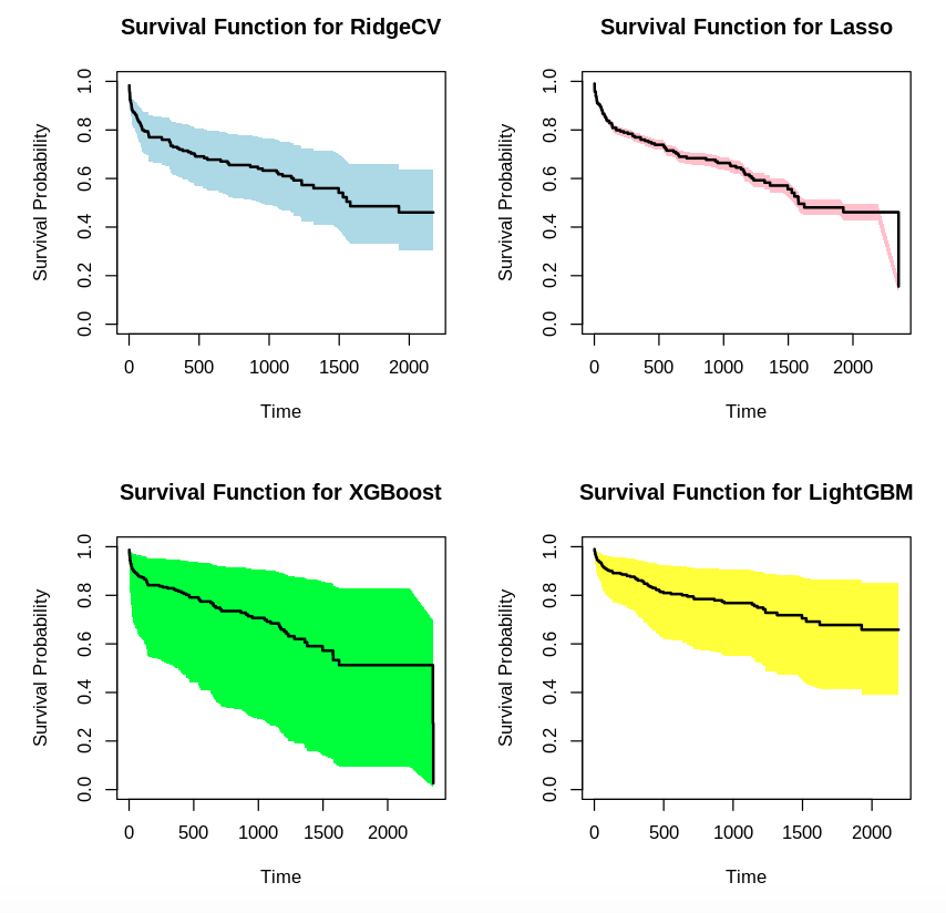
In this post, I show how to use scikit-learn, xgboost, lightgbm in R, in conjuction with Python package survivalist for probabilistic survival analysis. The probabilistic part is based on conformal prediction and Bayesian inference, and graphics represent the out-of-sample ML survival function.
utils::install.packages("reticulate")
library(reticulate)

# Install necessary Python packages (https://github.com/Techtonique/survivalist)
system("pip uninstall -y survivalist")
system("pip install survivalist --upgrade --no-cache-dir --verbose")

# Import Python modules (/!\ this will work if the Python packages are in the environment, e.g in Colab)
np <- import("numpy")
pd <- import("pandas")
lgb <- import("lightgbm")
xgb <- import("xgboost")
survivalist <- import("survivalist")
sklearn <- import("sklearn")
# Load specific functions
load_whas500 <- survivalist$datasets$load_whas500
PIComponentwiseGenGradientBoostingSurvivalAnalysis <- survivalist$ensemble$PIComponentwiseGenGradientBoostingSurvivalAnalysis
PISurvivalCustom <- survivalist$custom$PISurvivalCustom
RidgeCV <- sklearn$linear_model$RidgeCV
Lasso <- sklearn$linear_model$Lasso
XGB <- xgb$XGBRegressor
LGBM <- lgb$LGBMRegressor
train_test_split <- sklearn$model_selection$train_test_split

# Function for one-hot encoding categorical columns
encode_categorical_columns <- function(df, categorical_columns = NULL) {
  if (is.null(categorical_columns)) {
    categorical_columns <- names(df)[sapply(df, is.character)]
  }
  df_encoded <- py_to_r(pd$get_dummies(r_to_py(df), columns = categorical_columns))
  return(df_encoded)
}
# Load data
data <- load_whas500()
X <- py_to_r(data[[1]])
y <- py_to_r(data[[2]])
X <- encode_categorical_columns(X)
# Split into training and test sets
# Perform the split in Python to avoid unnecessary conversions
split_data <- train_test_split(r_to_py(X), r_to_py(y), test_size = 0.2, random_state = 42L)
X_train <- split_data[[1]] # Keep X_train as a Python object
X_test <- split_data[[2]]  # Keep X_test as a Python object
y_train <- split_data[[3]] # Keep y_train as a Python object
y_test <- split_data[[4]]  # Keep y_test as a Python object


# Survival model
# Fit the models using Python objects directly, and specifying the type of uncertainty
estimator1 <- PIComponentwiseGenGradientBoostingSurvivalAnalysis(regr=RidgeCV(), type_pi="bootstrap")
estimator1$fit(X_train, y_train)

estimator2 <- PIComponentwiseGenGradientBoostingSurvivalAnalysis(regr=Lasso(), type_pi="kde")
estimator2$fit(X_train, y_train)

# set a random seed
estimator3 <- PISurvivalCustom(regr=XGB(), type_pi="bootstrap")
estimator3$fit(X_train, y_train)

# set a random seed
estimator4 <- PISurvivalCustom(regr=LGBM(), type_pi="kde")
estimator4$fit(X_train, y_train)
PIComponentwiseGenGradientBoostingSurvivalAnalysis(regr=RidgeCV(),
                                                   type_pi='bootstrap')
PIComponentwiseGenGradientBoostingSurvivalAnalysis(regr=Lasso(), type_pi='kde')
PISurvivalCustom(regr=XGBRegressor(base_score=None, booster=None,
                                   callbacks=None, colsample_bylevel=None,
                                   colsample_bynode=None, colsample_bytree=None,
                                   device=None, early_stopping_rounds=None,
                                   enable_categorical=False, eval_metric=None,
                                   feature_types=None, gamma=None,
                                   grow_policy=None, importance_type=None,
                                   interaction_constraints=None,
                                   learning_rate=None, max_bin=None,
                                   max_cat_threshold=None,
                                   max_cat_to_onehot=None, max_delta_step=None,
                                   max_depth=None, max_leaves=None,
                                   min_child_weight=None, missing=nan,
                                   monotone_constraints=None,
                                   multi_strategy=None, n_estimators=None,
                                   n_jobs=None, num_parallel_tree=None,
                                   random_state=None, ...),
                 type_pi='bootstrap')
PISurvivalCustom(regr=LGBMRegressor(), type_pi='kde')
# Predict survival functions for an individual
# Use X_test as a Python object
surv_funcs <- estimator1$predict_survival_function(X_test[1, , drop = FALSE]) # Indexing in Python starts from 0
surv_funcs2 <- estimator2$predict_survival_function(X_test[1, , drop = FALSE]) # Indexing in Python starts from 0
surv_funcs3 <- estimator3$predict_survival_function(X_test[1, , drop = FALSE]) # Indexing in Python starts from 0
surv_funcs4 <- estimator4$predict_survival_function(X_test[1, , drop = FALSE]) # Indexing in Python starts from 0
# Extract survival function values
times <- surv_funcs$mean[[1]]$x
surv_prob <- surv_funcs$mean[[1]]$y
lower_bound <- surv_funcs$lower[[1]]$y
upper_bound <- surv_funcs$upper[[1]]$y

times2 <- surv_funcs2$mean[[1]]$x
surv_prob2 <- surv_funcs2$mean[[1]]$y
lower_bound2 <- surv_funcs2$lower[[1]]$y
upper_bound2 <- surv_funcs2$upper[[1]]$y

times3 <- surv_funcs3$mean[[1]]$x
surv_prob3 <- surv_funcs3$mean[[1]]$y
lower_bound3 <- surv_funcs3$lower[[1]]$y
upper_bound3 <- surv_funcs3$upper[[1]]$y

times4 <- surv_funcs4$mean[[1]]$x
surv_prob4 <- surv_funcs4$mean[[1]]$y
lower_bound4 <- surv_funcs4$lower[[1]]$y
upper_bound4 <- surv_funcs4$upper[[1]]$y

par(mfrow=c(2, 2))
plot(times, surv_prob, type = "s", ylim = c(0, 1), xlab = "Time", ylab = "Survival Probability", main = "Survival Function for RidgeCV")
polygon(c(times, rev(times)), c(lower_bound, rev(upper_bound)), col = "lightblue", border = NA)
lines(times, surv_prob, type = "s", lwd = 2)
plot(times2, surv_prob2, type = "s", ylim = c(0, 1), xlab = "Time", ylab = "Survival Probability", main = "Survival Function for Lasso")
polygon(c(times2, rev(times2)), c(lower_bound2, rev(upper_bound2)), col = "pink", border = NA)
lines(times2, surv_prob2, type = "s", lwd = 2)
plot(times3, surv_prob3, type = "s", ylim = c(0, 1), xlab = "Time", ylab = "Survival Probability", main = "Survival Function for XGBoost")
polygon(c(times3, rev(times3)), c(lower_bound3, rev(upper_bound3)), col = "green", border = NA)
lines(times3, surv_prob3, type = "s", lwd = 2)
plot(times4, surv_prob4, type = "s", ylim = c(0, 1), xlab = "Time", ylab = "Survival Probability", main = "Survival Function for LightGBM")
polygon(c(times4, rev(times4)), c(lower_bound4, rev(upper_bound4)), col = "yellow", border = NA)
lines(times4, surv_prob4, type = "s", lwd = 2)

Comments powered by Talkyard.