Last year, in a previous post,
I’ve used Python package the-teller to explain an xgboost model’s predictions.
After reading today’s post, you’ll be able to use that same package, the-teller, to explain
predictions of a Keras neural network trained on tabular data.
We start by installing the following tools:
- An AutoML system based on Keras:
pip install autokeras
It’s worth mentioning that I’m not using autokeras here to obtain a perfect model (try a Random Forest in the
same setting as the one described below ;) ). Rather,
I’m using it to obtain a relatively good Keras model without much manual tuning.
- General-purpose Statistical/Machine Learning tools:
pip install scikit-learn - A wrapper that allows to use Keras models as scikit-learn models (
fit,predict, model selection, pipelines, etc.):pip install scikeras - Scientific computing/data wrangling in Python:
pip install scipy==1.4.1pip install numpypip install pandas -
Tensorflow (Keras is built on top of this package)
- A tool for explaining predictions of Statistical/Machine Learning models on tabular data:
pip install the-teller
After the installation, we import these packages into Python:
import numpy as np
import pandas as pd
import autokeras as ak
import teller as tr

from sklearn.datasets import fetch_california_housing
from sklearn.metrics import mean_squared_error
from sklearn.model_selection import train_test_split
from scikeras.wrappers import KerasRegressor
The dataset used for this demo, the California housing dataset (imported by sklearn’s fetch_california_housing), has the following description:
- __Response__ / __target__ to be explained: median __house value for California districts__, in hundreds of thousands of dollars ($100,000)

- __MedInc__: median income in block group

- __HouseAge__: median house age in block group

- __AveRooms__: average number of rooms per household

- __AveBedrms__: average number of bedrooms per household

- __Population__: block group population

- __AveOccup__: average number of household members

- __Latitude__: block group latitude

- __Longitude__: block group longitude
# Input data from california housing
X, y = fetch_california_housing(return_X_y=True, as_frame=False)

# Columns names
X_names = fetch_california_housing(return_X_y=True, as_frame=True)[0].columns


# Split data into a training test and a test set
X_train, X_test, y_train, y_test = train_test_split(X, y,
                                                    test_size=0.2, random_state=13)
# Initialize autokeras's structured data regressor.
reg = ak.StructuredDataRegressor(
    overwrite=True, max_trials=100, loss="mean_squared_error",
)  # It tries 100 different models. Try a lower `max_trials` for a faster result.

# Feed the structured data regressor with training data, and train on 20 epochs.
reg.fit(x=X_train, y=y_train, epochs=20)

# Predict with the _best_ model found by autokeras.
predicted_y = reg.predict(X_test)

# Out-of-sample error (Root Mean Squared Error)
print(mean_squared_error(y_true=y_test, y_pred=predicted_y.flatten(), squared=False))
The model found by autokeras, reg, is exported to a Keras model, whose summary
of layers and parameters can be printed:
model = reg.export_model()
print(model.summary())
Model: "model"
_________________________________________________________________
 Layer (type)                Output Shape              Param #
=================================================================
 input_1 (InputLayer)        [(None, 8)]               0

 multi_category_encoding (Mu  (None, 8)                0
 ltiCategoryEncoding)

 normalization (Normalizatio  (None, 8)                17
 n)

 dense (Dense)               (None, 512)               4608

 re_lu (ReLU)                (None, 512)               0

 dense_1 (Dense)             (None, 1024)              525312

 re_lu_1 (ReLU)              (None, 1024)              0

 regression_head_1 (Dense)   (None, 1)                 1025

=================================================================
Total params: 530,962
Trainable params: 530,945
Non-trainable params: 17
Now that we have a Keras model, we can use a scikeras wrapper to obtain a
sklearn-like regressor (required by the-teller):
reg2 = KerasRegressor(
    model=model,
    loss="mse",
    metrics=[mean_squared_error],
)

reg2.fit(X_train, y_train)
All the ingredients for feeding the-teller’s Explainer are now gathered:
# creating the explainer
explainer = tr.Explainer(obj=reg2)

# fitting the explainer to unseen data
explainer.fit(X_test, y_test, X_names=X_names, method="avg")
explainer.plot(what="average_effects")
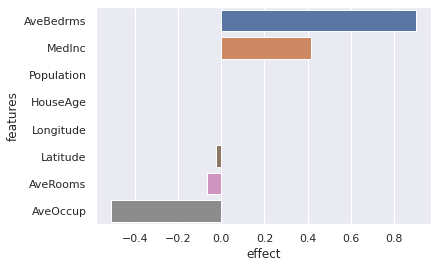
According to this Keras neural network, all else held equal, the average number of bedrooms and the median income in block are the most important drivers for an increase in housing value. Surprisingly too (or not?), when the housing age in block group is increased by a little \(\epsilon\), the housing value does not change on average – all else held equal.
explainer.summary()
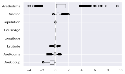
Heterogeneity of marginal effects:
                mean       std    median       min       max
AveBedrms   1.461185  1.491522  1.241837 -2.834498  7.180917
MedInc      0.412377  0.251765  0.394124 -0.215032  1.737655
Population  0.000037  0.000209  0.000026 -0.000666  0.001251
HouseAge    0.000000  0.000000  0.000000  0.000000  0.000000
Longitude   0.000000  0.000000 -0.000000 -0.000000 -0.000000
Latitude   -0.042189  0.164907 -0.039731 -0.743647  0.643677
AveRooms   -0.085101  0.228191 -0.056002 -0.938256  0.783281
AveOccup   -0.567745  0.487438 -0.422143 -2.381372  0.105577
Heterogeneity of marginal effects:
explainer.plot(what="hetero_effects")
Individual effects on the whole test set:
print(explainer.get_individual_effects())
       MedInc  HouseAge  AveRooms  AveBedrms  Population  AveOccup  Latitude  \
0     0.156049       0.0  0.184784   0.161584   -0.000261 -0.108461 -0.056902
1     0.667402       0.0  0.031313   4.240315   -0.000012 -1.353364  0.575099
2     1.190386       0.0 -0.524089   2.302171   -0.000037 -0.957003 -0.064196
3     0.184671       0.0  0.048120   0.186709    0.000074 -0.137837 -0.124834
4     0.297273       0.0 -0.282084   1.098558   -0.000015 -0.411185  0.053061
...        ...       ...       ...        ...         ...       ...       ...
4123 -0.052363       0.0  0.080290   0.521982   -0.000197 -0.678636  0.213984
4124  1.141179       0.0 -0.103344   3.325628    0.000310 -1.212456  0.199239
4125  0.314250       0.0 -0.406678   0.826998   -0.000032 -0.110662  0.045599
4126  0.354891       0.0  0.022459   0.639016    0.000046 -0.280295 -0.103073
4127  0.274952       0.0 -0.089247   0.888977    0.000013 -0.297384  0.239034

      Longitude
0          -0.0
1          -0.0
2          -0.0
3          -0.0
4          -0.0
...         ...
4123       -0.0
4124       -0.0
4125       -0.0
4126       -0.0
4127       -0.0

[4128 rows x 8 columns]