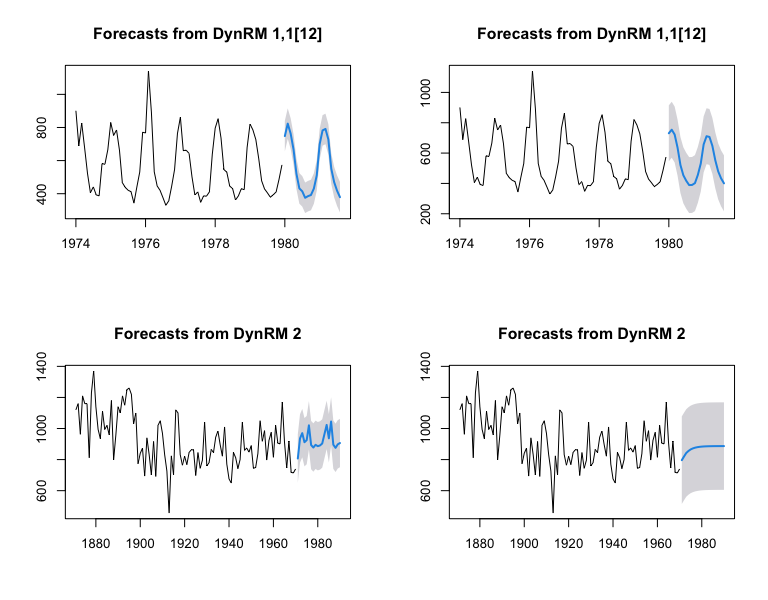
A few weeks ago, I introduced the R version of ahead, a package for univariate and multivariate time series forecasting. A Python version, built on top of the R version, is now available on PyPI and GitHub. Here is how to install it:
-
1st method: from PyPI (stable version)
pip install ahead -
2nd method: from Github (development version)
pip install git+https://github.com/Techtonique/ahead_python.git
Here are the packages that will be used for this demo:
import pandas as pd # for creating Python time series data structures
import ahead as ah # might take some time installing R packages, ONLY the 1st time it's called
Univariate time series forecasting
# Input time series
dataset = {
'date' : ['2020-01-01', '2020-02-01', '2020-03-01', '2020-04-01', '2020-05-01',
'2020-06-01', '2020-07-01', '2020-08-01', '2020-09-01', '2020-10-01'],
'value' : [34, 30, 35.6, 33.3, 38.1, 39.2, 37.3, 34.5, 35.6, 35.9]}

# Data frame containing the time series
df = pd.DataFrame(dataset).set_index('date')

# For more details on EAT class parameters, visit
# https://techtonique.github.io/ahead_python/documentation/eat/
e1 = ah.EAT(h = 5)
e1.forecast(df)
print(e1.result_df_)
                 mean      lower      upper
2020-11-01  35.995003  30.538903  41.451110
2020-12-01  36.059549  30.603449  41.515655
2021-01-01  36.124094  30.667994  41.580201
2021-02-01  36.188640  30.732540  41.644746
2021-03-01  36.253185  30.797085  41.709292
Multivariate time series forecasting
# Input time series
dataset = {
 'date' : ['2001-01-01', '2002-01-01', '2003-01-01', '2004-01-01', '2005-01-01'],
 'series1' : [34, 30, 35.6, 33.3, 38.1],
 'series2' : [4, 5.5, 5.6, 6.3, 5.1],
 'series3' : [100, 100.5, 100.6, 100.2, 100.1]}

# Data frame containing the (3) time series
df = pd.DataFrame(dataset).set_index('date')

# For more details on Ridge2Regressor class parameters, visit
# https://techtonique.github.io/ahead_python/documentation/ridge2regressor/
r1 = ah.Ridge2Regressor(h = 5)
r1.forecast(df)
print(r1.result_dfs_[0])
print(r1.result_dfs_[1])
print(r1.result_dfs_[2])
                 mean      lower      upper
2006-01-01  33.995386  33.927846  34.062925
2007-01-01  36.801638  36.734099  36.869178
2008-01-01  33.080255  33.012716  33.147795
2009-01-01  36.101237  36.033697  36.168777
2010-01-01  33.584086  33.516547  33.651626
                mean     lower     upper
2006-01-01  5.488425  5.474439  5.502412
2007-01-01  4.891770  4.877784  4.905756
2008-01-01  5.536466  5.522480  5.550452
2009-01-01  5.187249  5.173263  5.201236
2010-01-01  5.680144  5.666158  5.694130
                  mean       lower       upper
2006-01-01   99.936592   99.929847   99.943337
2007-01-01  100.110577  100.103832  100.117322
2008-01-01  100.097996  100.091251  100.104741
2009-01-01  100.235343  100.228598  100.242089
2010-01-01  100.136356  100.129611  100.143101

