Due to the way it mixes several – relatively – simple concepts, Bayesian optimization (BO) is one of the most elegant mathematical tool I’ve encountered so far. In this post, I introduce GPopt, a tool for BO that I implemented in Python (no technical docs yet, but coming soon). The examples of GPopt’s use showcased here are based on Gaussian Processes (GP) and Expected Improvement (EI): what does that mean?
GPs are Bayesian statistical/machine learning (ML) models which create a distribution on functions, and especially on black-box functions. If we let \(f\) be the black-box – and expensive-to-evaluate – function whose minimum is searched, a GP is firstly adjusted (in a supervised learning way) to a small set of points at which \(f\) is evaluated. This small set of points is the initial design. Then the GP, thanks to its probabilistic nature, will exploit its knowledge of previous points at which \(f\) has already been evaluated, to explore new points: potential minimas maximizing an EI criterion. It’s a reinforcement learning question!
For more details on Bayesian optimization applied to hyperparameters calibration in ML, you can read Chapter 6 of this document. In this post, a Branin (2D) and a Hartmann (3D) functions will be used as examples of objective functions \(f\), and Matérn 5/2 is the GP’s covariance.
Installing and importing the packages:
!pip install GPopt
!pip install matplotlib==3.1.3
import GPopt as gp
import time
import sys
import numpy as np
import matplotlib.pyplot as plt
from os import chdir
from scipy.optimize import minimize
The objective function to be minimized:
# branin function
def branin(x):
    x1 = x[0]
    x2 = x[1]
    term1 = (x2 - (5.1*x1**2)/(4*np.pi**2) + (5*x1)/np.pi - 6)**2
    term2 = 10*(1-1/(8*np.pi))*np.cos(x1)
    return (term1 + term2 + 10)
# A local minimum for verification
print("\n")
res = minimize(branin, x0=[0, 0], method='Nelder-Mead', tol=1e-6)
print(res.x)
print(branin(res.x))
[3.14159271 2.27500017]
0.397887357729795
Firstly, I demonstrate the convergence of the optimizer towards a minimum (and show that the optimizer can pick up the procedure where it left):
# n_init is the number of points in the initial design
# n_iter is the number of iterations of the optimizer
gp_opt = gp.GPOpt(objective_func=branin,
                lower_bound = np.array([-5, 0]),
                 upper_bound = np.array([10, 15]),
                 n_init=10, n_iter=10)
gp_opt.optimize(verbose=1)
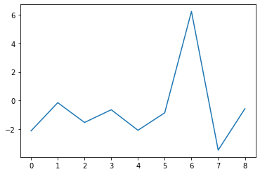
Plotting the changes in expected improvement as a function of the number of iterations.
print(gp_opt.x_min) # current minimum
print(gp_opt.y_min) # current minimum
plt.plot(np.diff(gp_opt.max_ei))
[9.31152344 1.68457031]
0.9445903336427559
Adding more iterations to the optimizer:
gp_opt.optimize(verbose=1, n_more_iter=10)
 ...Done.


 Optimization loop...

10/10 [██████████████████████████████] - 2s 186ms/step

(array([3.22692871, 2.63122559]), 0.6107733232129569)
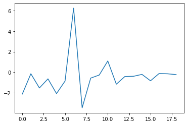
Plotting the changes in expected improvement as a function of the number of iterations (again).
print(gp_opt.x_min) # current minimum
print(gp_opt.y_min) # current minimum
plt.plot(np.diff(gp_opt.max_ei))
[3.22692871 2.63122559]
0.6107733232129569
Adding more iterations to the optimizer (again):
gp_opt.optimize(verbose=1, n_more_iter=80)
Plotting the changes in expected improvement as a function of the number of iterations (again).
print(gp_opt.x_min) # current minimum
print(gp_opt.y_min) # current minimum
plt.plot(np.diff(gp_opt.max_ei))
[9.44061279 2.48199463]
0.3991320518189241
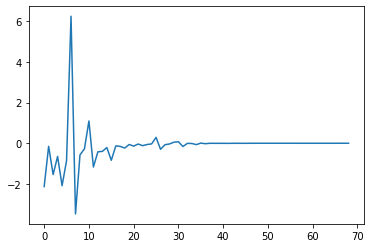
The 3 previous graphs suggest the possibility of stopping the optimizer earlier, when the algorithm is not improving on previous points’ results anymore:
# # early stopping
# abs_tol is the parameter that controls early stopping

gp_opt2 = gp.GPOpt(objective_func=branin,
                  lower_bound = np.array([-5, 0]),
                 upper_bound = np.array([10, 15]),
                 n_init=10, n_iter=190)
gp_opt2.optimize(verbose=2, abs_tol=1e-4)
print("\n")
We can observe that only 58 iterations are necessary when abs_tol = 1e-4
print(gp_opt2.n_iter)
print(gp_opt2.x_min)
print(gp_opt2.y_min)
58
[9.44061279 2.48199463]
0.3991320518189241
Illustrating convergence:
plt.plot(gp_opt2.max_ei)
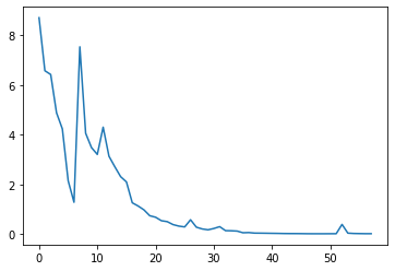
We notice that in this example, GPopt falls into a local minimum but is very close to the previous minimum found with gradient-free optimizer (Nelder-Mead). The opposite situation can occur too:
# [0, 1]^3
def hartmann3(xx):

    alpha = np.array([1.0, 1.2, 3.0, 3.2])

    A = np.array([3.0, 10, 30,
                  0.1, 10, 35,
                  3.0, 10, 30,
                  0.1, 10, 35]).reshape(4, 3)

    P = 1e-4 * np.array([3689, 1170, 2673,
                        4699, 4387, 7470,
                        1091, 8732, 5547,
                        381, 5743, 8828]).reshape(4, 3)

    xxmat = np.tile(xx,4).reshape(4, 3)

    inner = np.sum(A*(xxmat-P)**2, axis = 1)
    outer = np.sum(alpha * np.exp(-inner))

    return(-outer)
# Fails, but may work with multiple restarts
print("\n")
res = minimize(hartmann3, x0=[0, 0, 0], method='Nelder-Mead', tol=1e-6)
print(res.x)
print(hartmann3(res.x))
[0.36872308 0.11756145 0.26757363]
-1.00081686355956
# hartmann 3D
gp_opt4 = gp.GPOpt(objective_func=hartmann3,
                lower_bound = np.repeat(0, 3),
                upper_bound = np.repeat(1, 3),
                 n_init=20, n_iter=280)
gp_opt4.optimize(verbose=2, abs_tol=1e-4)
print(gp_opt4.n_iter)
print(gp_opt4.x_min)
print(gp_opt4.y_min)
print("\n")
51
[0.07220459 0.55792236 0.85662842]
-3.8600590626769904
The question is, in the case of BO applied to ML cross-validation, do we really want to find the global minimum of the objective function?