Sometimes in Statistical/Machine Learning problems, we encounter categorical explanatory variables with high cardinality. Let’s say for example that we want to determine if a diet is good or bad, based on what a person eats. In trying to answer this question, we’d construct a response variable containing a sequence of characters good or bad, one for each person; and an explanatory variable for the model would be:
x = c("apple", "tomato", "banana", "apple", "pineapple", "bic mac",
	"banana", "bic mac", "quinoa sans gluten", "pineapple",
	"avocado", "avocado", "avocado", "avocado!", ...)
Some Statistical/Machine learning models only accept numerical data as input. Hence the need for a way to transform those categorical inputs into numerical vectors. One way to deal with a covariate such as x is to use one-hot encoding, as depicted below:
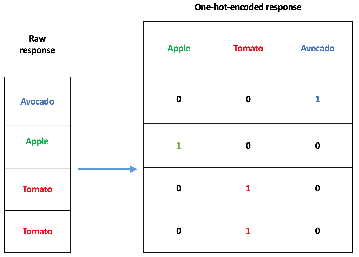
In the case of x having 100 types of fruits in it, one-hot encoding will lead to 99 explanatory variables for the model, instead of, possibly one. This means: more disk space required, more computer memory needed, and a longer training time. Apart from the one-hot encoder, there are a lot of categorical encoders out there. I wanted a relatively simple one, so I came up with the one described in this post. It’s a target-based categorical encoder, which makes use of the correlation between a randomly generated pseudo-target and the real target (a.k.a response; a sequence good or bads as seen before).
Data and packages for the demo
We’ll be using the CO2 dataset available in base R for this demo. According to its description: the CO2 data frame has 84 rows and 5 columns of data from an experiment on the cold tolerance of the grass species Echinochloa crus-gall.
# Packages required
library(randomForest)

# Dataset
Xy <- datasets::CO2
Xy$uptake <- scale(Xy$uptake) # centering and scaling the response
print(dim(Xy))
print(head(Xy))
print(tail(Xy))
Now we create a response variables and covariates, based on CO2 data:
y <- Xy$uptake
X <- Xy[, c("Plant", "Type", "Treatment" ,"conc")]
First encoder: “One-hot”
Using base R’s function model.matrix, we transform the categorical variables from CO2 to numerical variables. It’s not exactly “One-hot” as we described it previously, but a close cousin, because the covariate Plant possesses some sort of ordering (it’s “an ordered factor with levels Qn1 < Qn2 < Qn3 < … < Mc1 giving a unique identifier for each plant”):
X_onehot <- model.matrix(uptake ~ ., data=CO2)[,-1]
print(dim(X_onehot))
print(head(X_onehot))
print(tail(X_onehot))
## [1] 84 14

##      Plant.L   Plant.Q    Plant.C   Plant^4    Plant^5   Plant^6
## 1 -0.4599331 0.5018282 -0.4599331 0.3687669 -0.2616083 0.1641974
## 2 -0.4599331 0.5018282 -0.4599331 0.3687669 -0.2616083 0.1641974
## 3 -0.4599331 0.5018282 -0.4599331 0.3687669 -0.2616083 0.1641974
## 4 -0.4599331 0.5018282 -0.4599331 0.3687669 -0.2616083 0.1641974
## 5 -0.4599331 0.5018282 -0.4599331 0.3687669 -0.2616083 0.1641974
## 6 -0.4599331 0.5018282 -0.4599331 0.3687669 -0.2616083 0.1641974
##       Plant^7    Plant^8     Plant^9    Plant^10     Plant^11
## 1 -0.09047913 0.04307668 -0.01721256 0.005456097 -0.001190618
## 2 -0.09047913 0.04307668 -0.01721256 0.005456097 -0.001190618
## 3 -0.09047913 0.04307668 -0.01721256 0.005456097 -0.001190618
## 4 -0.09047913 0.04307668 -0.01721256 0.005456097 -0.001190618
## 5 -0.09047913 0.04307668 -0.01721256 0.005456097 -0.001190618
## 6 -0.09047913 0.04307668 -0.01721256 0.005456097 -0.001190618
##   TypeMississippi Treatmentchilled conc
## 1               0                0   95
## 2               0                0  175
## 3               0                0  250
## 4               0                0  350
## 5               0                0  500
## 6               0                0  675

##      Plant.L   Plant.Q    Plant.C    Plant^4    Plant^5    Plant^6
## 79 0.3763089 0.2281037 -0.0418121 -0.3017184 -0.4518689 -0.4627381
## 80 0.3763089 0.2281037 -0.0418121 -0.3017184 -0.4518689 -0.4627381
## 81 0.3763089 0.2281037 -0.0418121 -0.3017184 -0.4518689 -0.4627381
## 82 0.3763089 0.2281037 -0.0418121 -0.3017184 -0.4518689 -0.4627381
## 83 0.3763089 0.2281037 -0.0418121 -0.3017184 -0.4518689 -0.4627381
## 84 0.3763089 0.2281037 -0.0418121 -0.3017184 -0.4518689 -0.4627381
##       Plant^7    Plant^8    Plant^9    Plant^10   Plant^11 TypeMississippi
## 79 -0.3701419 -0.2388798 -0.1236175 -0.04910487 -0.0130968               1
## 80 -0.3701419 -0.2388798 -0.1236175 -0.04910487 -0.0130968               1
## 81 -0.3701419 -0.2388798 -0.1236175 -0.04910487 -0.0130968               1
## 82 -0.3701419 -0.2388798 -0.1236175 -0.04910487 -0.0130968               1
## 83 -0.3701419 -0.2388798 -0.1236175 -0.04910487 -0.0130968               1
## 84 -0.3701419 -0.2388798 -0.1236175 -0.04910487 -0.0130968               1
##    Treatmentchilled conc
## 79                1  175
## 80                1  250
## 81                1  350
## 82                1  500
## 83                1  675
## 84                1 1000
Second encoder: Target-based
Now, we present the encoder discussed in the introduction. It’s a target-based categorical encoder, which uses the correlation between a randomly generated pseudo-target and the real target.
Construction of a pseudo-target via Cholesky decomposition
Most target encoders rely directly on the response variable, which leads to a potential risk called leakage. Target encoding is indeed a form of more or less subtle overfitting. Here, in order to somehow circumvent this issue, we use Cholesky decomposition. We create a pseudo-target based on the real target uptake (centered and scaled, and stored in variable y), and specifically ask that, this pseudo-target has a fixed correlation of -0.4 (could be anything) with the response:
# reproducibility seed
set.seed(518)

# target covariance matrix
rho <- -0.4 # desired target
C <- matrix(rep(rho, 4), nrow = 2, ncol = 2)
diag(C) <- 1

# Cholesky decomposition
(C_ <- chol(C))
print(t(C_)%*%C_)

X2 <- rnorm(n)
XX <- cbind(y, X2)

# induce correlation through Cholesky decomposition
X_ <- XX %*% C_
colnames(X_) <- c("real_target", "pseudo_target")
Print the induced correlation between the randomly generated pseudo-target and the real target:
cor(y, X_[,2])
##            [,1]
## [1,] -0.4008563
Now, a glimpse at X_, a matrix containing the real target and the pseudo target in columns:
print(dim(X_))
print(head(X_))
print(tail(X_))
## [1] 84  2

##      real_target pseudo_target
## [1,]  -1.0368659    -0.6668123
## [2,]   0.2946905     0.3894672
## [3,]   0.7015550     0.3485984
## [4,]   0.9234810    -1.2769424
## [5,]   0.7477896    -1.1996023
## [6,]   1.1084194     0.4008157

##       real_target pseudo_target
## [79,]  -0.8519275    -0.3455701
## [80,]  -0.8611744     1.7142739
## [81,]  -0.8611744     0.1521795
## [82,]  -0.8611744    -0.3912856
## [83,]  -0.7687052     0.9726421
## [84,]  -0.6762360     0.8791499
A few checks
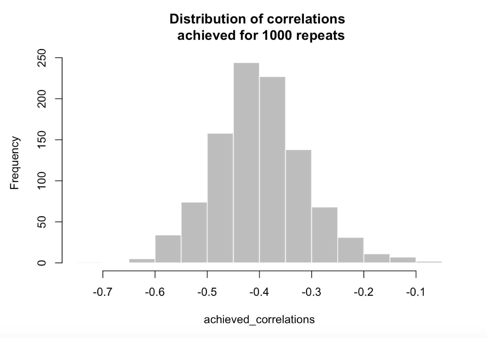
By repeating the procedure that we just outlined with 1000 seeds going from 1 to 1000, we obtain a distribution of achieved correlations between the real target and the pseudo target:
## $breaks
##  [1] -0.75 -0.70 -0.65 -0.60 -0.55 -0.50 -0.45 -0.40 -0.35 -0.30 -0.25
## [12] -0.20 -0.15 -0.10 -0.05
##
## $counts
##  [1]   1   0   5  34  74 158 244 227 138  68  31  11   7   2
##
## $density
##  [1] 0.02 0.00 0.10 0.68 1.48 3.16 4.88 4.54 2.76 1.36 0.62 0.22 0.14 0.04
##
## $mids
##  [1] -0.725 -0.675 -0.625 -0.575 -0.525 -0.475 -0.425 -0.375 -0.325 -0.275
## [11] -0.225 -0.175 -0.125 -0.075
##
## $xname
## [1] "achieved_correlations"
##
## $equidist
## [1] TRUE
##
## attr(,"class")
## [1] "histogram"
print(summary(achieved_correlations))
##     Min.  1st Qu.   Median     Mean  3rd Qu.     Max.
## -0.70120 -0.45510 -0.40270 -0.40040 -0.34820 -0.08723
Encoding
In order to encode the factors, we use the pseudo-target y_ defined as:
y_ <- X_[ , 'pseudo_target']
Our new, numerically encoded covariates are derived by calculating sums of the pseudo-target y_ (we could think of other types of aggregations), groupped by factor level for each factor. The new matrix of covariates is named X_Cholesky:
print(dim(X_Cholesky))
print(head(X_Cholesky))
print(tail(X_Cholesky))
## [1] 84  4

##          Plant      Type Treatment conc
## [1,] -1.853112 -18.08574 -7.508514   95
## [2,] -1.853112 -18.08574 -7.508514  175
## [3,] -1.853112 -18.08574 -7.508514  250
## [4,] -1.853112 -18.08574 -7.508514  350
## [5,] -1.853112 -18.08574 -7.508514  500
## [6,] -1.853112 -18.08574 -7.508514  675

##          Plant     Type  Treatment conc
## [79,] 2.628531 9.658954 -0.9182766  175
## [80,] 2.628531 9.658954 -0.9182766  250
## [81,] 2.628531 9.658954 -0.9182766  350
## [82,] 2.628531 9.658954 -0.9182766  500
## [83,] 2.628531 9.658954 -0.9182766  675
## [84,] 2.628531 9.658954 -0.9182766 1000
Notice that X_Cholesky has 4 covariates, that X_onehot had 14 covariates, and imagine a situation with a higher cardinality for each factor.
Fit a model to one-hot encoded and target based covariates
In this section, we compare both types of encoding using cross-validation with Root Mean Squared Errors (RMSE).
Datasets
# Dataset with one-hot encoded covariates
Xy1 <- data.frame(y, X_onehot)

# Dataset with pseudo-target-based encoding of covariates
Xy2 <- data.frame(y, X_Cholesky)
Comparison
Using a Random Forest here as a simple illustration without hyperparameter tuning, but tree-based models will typically handle this type of data. Not linear models, nor Neural Networks or Support Vector Machines.
Random Forests with 100 seeds, going from 1 to 100 are adjusted:
n_reps <- 100
n_train <- length(y)
`%op%` <- foreach::`%do%`
pb <- utils::txtProgressBar(min=0, max=n_reps, style = 3)
errs <- foreach::foreach(i = 1:n_reps, .combine=rbind)%op%
{
 # utils::setTxtProgressBar(pb, i)
  set.seed(i)
  index_train <- sample.int(n_train, size = floor(0.8*n_train))
  obj1 <- randomForest(y ~ ., data=Xy1[index_train, ])
  obj2 <- randomForest(y ~ ., data=Xy2[index_train, ])
  c(sqrt(mean((predict(obj1, newdata=as.matrix(Xy1[-index_train, -1])) - y[-index_train])^2)),
   sqrt(mean((predict(obj2, newdata=as.matrix(Xy2[-index_train, -1])) - y[-index_train])^2)))
}
close(pb)
colnames(errs) <- c("one-hot", "target-based")
print(colMeans(errs))
print(apply(errs, 2, sd))
print(sapply(1:2, function (j) summary(errs[,j])))
##      one-hot target-based
##    0.4121657    0.4574857

##      one-hot target-based
##   0.09710344   0.07584037

##           [,1]   [,2]
## Min.    0.1877 0.2850
## 1st Qu. 0.3566 0.4039
## Median  0.4037 0.4464
## Mean    0.4122 0.4575
## 3rd Qu. 0.4784 0.4913
## Max.    0.6470 0.6840
There are certainly some improvements to be brought to this methodology, but the results discussed in this post already look quite encouraging to me.
Note: I am currently looking for a gig. You can hire me on Malt or send me an email: thierry dot moudiki at pm dot me. I can do descriptive statistics, data preparation, feature engineering, model calibration, training and validation, and model outputs’ interpretation. I am fluent in Python, R, SQL, Microsoft Excel, Visual Basic (among others) and French. My résumé? Here!

Under License Creative Commons Attribution 4.0 International.